Transfer Functions

This example demonstrates how to visualize the related transfer functions of the analog system and digital estimator.

import matplotlib.pyplot as plt
import numpy as np
import cbadc

Chain-of-Integrators ADC Example

In this example, we will use the chain-of-integrators ADC analog system for demonstrational purposes. However, except for the analog system creation, the steps for a generic analog system and digital estimator.

For in-depth details regarding the chain-of-integrators transfer function see, chain-of-integrators

First we will import dependent modules and initialize a chain-of-integrators setup. With the following analog system parameters

• \(\beta = \beta_1 = \dots = \beta_N = 6250\)

• \(\rho_1 = \dots = \rho_N = - 0.02\)

• \(\kappa_1 = \dots = \kappa_N = - 1\)

• \(N = 6\)

note that \(\mathbf{C}^\mathsf{T}\) is automatically assumed an identity matrix of size \(N\times N\).

Using the cbadc.analog_system.ChainOfIntegrators class which derives from the main analog system class cbadc.analog_system.AnalogSystem.

# We fix the number of analog states.
N = 6
# Set the amplification factor.
beta = 6250.
rho = - 0.02
kappa = - 1.0
# In this example, each nodes amplification and local feedback will be set
# identically.
betaVec = beta * np.ones(N)
rhoVec = betaVec * rho
kappaVec = kappa * beta * np.eye(N)

# Instantiate a chain-of-integrators analog system.
analog_system = cbadc.analog_system.ChainOfIntegrators(betaVec, rhoVec, kappaVec)
# print the system matrices.
print(analog_system)

Out:

The analog system is parameterized as:
A =
[[-125.    0.    0.    0.    0.    0.]
 [6250. -125.    0.    0.    0.    0.]
 [   0. 6250. -125.    0.    0.    0.]
 [   0.    0. 6250. -125.    0.    0.]
 [   0.    0.    0. 6250. -125.    0.]
 [   0.    0.    0.    0. 6250. -125.]],
B =
[[6250.]
 [   0.]
 [   0.]
 [   0.]
 [   0.]
 [   0.]],
CT =
[[1. 0. 0. 0. 0. 0.]
 [0. 1. 0. 0. 0. 0.]
 [0. 0. 1. 0. 0. 0.]
 [0. 0. 0. 1. 0. 0.]
 [0. 0. 0. 0. 1. 0.]
 [0. 0. 0. 0. 0. 1.]],
Gamma =
[[-6250.    -0.    -0.    -0.    -0.    -0.]
 [   -0. -6250.    -0.    -0.    -0.    -0.]
 [   -0.    -0. -6250.    -0.    -0.    -0.]
 [   -0.    -0.    -0. -6250.    -0.    -0.]
 [   -0.    -0.    -0.    -0. -6250.    -0.]
 [   -0.    -0.    -0.    -0.    -0. -6250.]],
Gamma_tildeT =
[[1. 0. 0. 0. 0. 0.]
 [0. 1. 0. 0. 0. 0.]
 [0. 0. 1. 0. 0. 0.]
 [0. 0. 0. 1. 0. 0.]
 [0. 0. 0. 0. 1. 0.]
 [0. 0. 0. 0. 0. 1.]], and D=[[0.]
 [0.]
 [0.]
 [0.]
 [0.]
 [0.]]

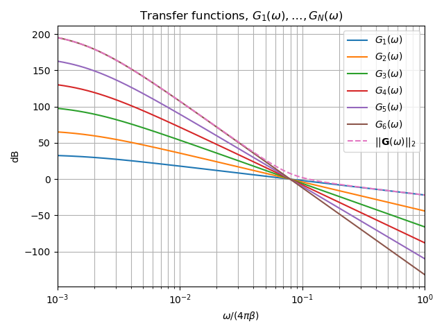
Plotting the Analog System’s Transfer Function

Next, we plot the transfer function of the analog system

\(\mathbf{G}(\omega) = \begin{pmatrix}G_1(\omega), \dots, G_N(\omega)\end{pmatrix}^\mathsf{T} = \mathbf{C}^\mathsf{T} \left(i \omega \mathbf{I}_N - \mathbf{A}\right)^{-1}\mathbf{B}\)

using the class method cbadc.analog_system.AnalogSystem.transfer_function_matrix().

# Logspace frequencies
frequencies = np.logspace(-3, 0, 500)
omega = 4 * np.pi * beta * frequencies

# Compute transfer functions for each frequency in frequencies
transfer_function = analog_system.transfer_function_matrix(omega)
transfer_function_dB = 20 * np.log10(np.abs(transfer_function))

# For each output 1,...,N compute the corresponding tranfer function seen
# from the input.
for n in range(N):
    plt.semilogx(
        frequencies, transfer_function_dB[n, 0, :], label=f"$G_{n+1}(\omega)$")

# Add the norm ||G(omega)||_2
plt.semilogx(
    frequencies,
    20 * np.log10(np.linalg.norm(
        transfer_function[:, 0, :],
        axis=0)),
    '--',
    label="$ ||\mathbf{G}(\omega)||_2 $")

# Add labels and legends to figure
plt.legend()
plt.grid(which='both')
plt.title("Transfer functions, $G_1(\omega), \dots, G_N(\omega)$")
plt.xlabel("$\omega / (4 \pi \\beta ) $")
plt.ylabel("dB")
plt.xlim((frequencies[0], frequencies[-1]))
plt.gcf().tight_layout()

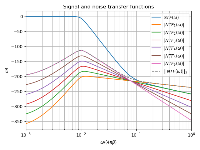
Plotting the Estimator’s Signal and Noise Transfer Function

To determine the estimate’s signal and noise transfer function, we must instantiate a digital estimator cbadc.digital_estimator.DigitalEstimator. The bandwidth of the digital estimation filter is mainly determined by the parameter \(\eta^2\) as the noise transfer function (NTF) follows as

\(\text{NTF}( \omega) = \mathbf{G}( \omega)^\mathsf{H} \left( \mathbf{G}( \omega)\mathbf{G}( \omega)^\mathsf{H} + \eta^2 \mathbf{I}_N \right)^{-1}\)

and similarly, the signal transfer function (STF) follows as

\(\text{STF}( \omega) = \text{NTF}( \omega) \mathbf{G}( \omega)\).

We compute these two by invoking the class methods cbadc.digital_estimator.DigitalEstimator.noise_transfer_function() and cbadc.digital_estimator.DigitalEstimator.signal_transfer_function() respectively.

the digital estimator requires us to also instantiate a digital control cbadc.digital_control.DigitalControl.

For the chain-of-integrators example, the noise transfer function results in a row vector \(\text{NTF}(\omega) = \begin{pmatrix} \text{NTF}_1(\omega), \dots, \text{NTF}_N(\omega)\end{pmatrix} \in \mathbb{C}^{1 \times \tilde{N}}\) where \(\text{NTF}_\ell(\omega)\) refers to the noise transfer function from the \(\ell\)-th observation to the final estimate.

# Define dummy control and control sequence (not used when computing transfer
# functions). However necessary to instantiate the digital estimator

T = 1/(2 * beta)
digital_control = cbadc.digital_control.DigitalControl(T, N)


# Compute eta2 for a given bandwidth.
omega_3dB = (4 * np.pi * beta) / 100.
eta2 = np.linalg.norm(analog_system.transfer_function_matrix(
    np.array([omega_3dB])).flatten()) ** 2

# Instantiate estimator.
digital_estimator = cbadc.digital_estimator.DigitalEstimator(
    analog_system, digital_control, eta2, K1=1)

# Compute NTF
ntf = digital_estimator.noise_transfer_function(omega)
ntf_dB = 20 * np.log10(np.abs(ntf))

# Compute STF
stf = digital_estimator.signal_transfer_function(omega)
stf_dB = 20 * np.log10(np.abs(stf.flatten()))


# Plot
plt.figure()
plt.semilogx(frequencies, stf_dB, label='$STF(\omega)$')
for n in range(N):
    plt.semilogx(frequencies, ntf_dB[0, n, :], label=f"$|NTF_{n+1}(\omega)|$")
plt.semilogx(frequencies, 20 * np.log10(np.linalg.norm(
    ntf[0, :, :], axis=0)), '--', label="$ || NTF(\omega) ||_2 $")

# Add labels and legends to figure
plt.legend()
plt.grid(which='both')
plt.title("Signal and noise transfer functions")
plt.xlabel("$\omega / (4 \pi \\beta ) $")
plt.ylabel("dB")
plt.xlim((frequencies[0], frequencies[-1]))
plt.gcf().tight_layout()

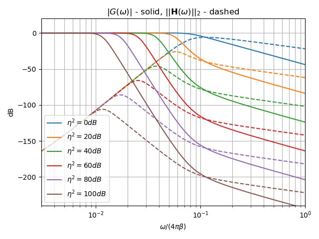
Setting the Bandwidth of the Estimation Filter

Finally, we will investigate the effect of eta2 on the STF and NTF.

# create a vector of etas to be evaluated,
eta2_vec = np.logspace(0, 10, 11)[::2]

plt.figure()
for eta2 in eta2_vec:
    # Instantiate an estimator for each eta.
    digital_estimator = cbadc.digital_estimator.DigitalEstimator(
        analog_system, digital_control, eta2, K1=1)
    # Compute stf and ntf
    ntf = digital_estimator.noise_transfer_function(omega)
    ntf_dB = 20 * np.log10(np.abs(ntf))
    stf = digital_estimator.signal_transfer_function(omega)
    stf_dB = 20 * np.log10(np.abs(stf.flatten()))

    # Plot
    color = next(plt.gca()._get_lines.prop_cycler)['color']
    plt.semilogx(frequencies, 20 *
                 np.log10(np.linalg.norm(ntf[0, :, :], axis=0)),
                 '--', color=color)
    plt.semilogx(frequencies, stf_dB,
                 label=f"$\eta^2={10 * np.log10(eta2):0.0f} dB$", color=color)

# Add labels and legends to figure
plt.legend(loc='lower left')
plt.grid(which='both')
plt.title("$|G(\omega)|$ - solid, $||\mathbf{H}(\omega)||_2$ - dashed")
plt.xlabel("$\omega / (4 \pi \\beta ) $")
plt.ylabel("dB")
plt.xlim((3e-3, 1))
plt.ylim((-240, 20))
plt.gcf().tight_layout()

Out:

/drives1/PhD/cbadc/docs/code_examples/a_getting_started/plot_d_transfer_function.py:196: RuntimeWarning: divide by zero encountered in log10
  ntf_dB = 20 * np.log10(np.abs(ntf))
/drives1/PhD/cbadc/docs/code_examples/a_getting_started/plot_d_transfer_function.py:196: RuntimeWarning: divide by zero encountered in log10
  ntf_dB = 20 * np.log10(np.abs(ntf))
/drives1/PhD/cbadc/docs/code_examples/a_getting_started/plot_d_transfer_function.py:196: RuntimeWarning: divide by zero encountered in log10
  ntf_dB = 20 * np.log10(np.abs(ntf))