Note
Click here to download the full example code
Digital Estimation
Converting a stream of control signals into a estimate samples.
 7 from cbadc.utilities import compute_power_spectral_density
 8 import matplotlib.pyplot as plt
 9 import cbadc
10 import numpy as np
Setting up the Analog System and Digital Control
In this example, we assume that we have access to a control signal s[k] generated by the interactions of an analog system and digital control. Furthermore, we assume a chain-of-integrators converter with corresponding analog system and digital control.

26 # Setup analog system and digital control
27
28 N = 6
29 M = N
30 beta = 6250.
31 rho = - 1e-2
32 kappa = - 1.0
33 A = [[beta * rho, 0, 0, 0, 0, 0],
34      [beta, beta * rho, 0, 0, 0, 0],
35      [0, beta, beta * rho, 0, 0, 0],
36      [0, 0, beta, beta * rho, 0, 0],
37      [0, 0, 0, beta, beta * rho, 0],
38      [0, 0, 0, 0, beta, beta * rho]]
39 B = [[beta], [0], [0], [0], [0], [0]]
40 CT = np.eye(N)
41 Gamma = [[kappa * beta, 0, 0, 0, 0, 0],
42          [0, kappa * beta, 0, 0, 0, 0],
43          [0, 0, kappa * beta, 0, 0, 0],
44          [0, 0, 0, kappa * beta, 0, 0],
45          [0, 0, 0, 0, kappa * beta, 0],
46          [0, 0, 0, 0, 0, kappa * beta]]
47 Gamma_tildeT = np.eye(N)
48 T = 1.0/(2 * beta)
49
50 analog_system = cbadc.analog_system.AnalogSystem(A, B, CT, Gamma, Gamma_tildeT)
51 digital_control = cbadc.digital_control.DigitalControl(T, M)
52
53 # Summarize the analog system, digital control, and digital estimator.
54 print(analog_system, "\n")
55 print(digital_control)
Out:
The analog system is parameterized as:
A =
[[ -62.5    0.     0.     0.     0.     0. ]
 [6250.   -62.5    0.     0.     0.     0. ]
 [   0.  6250.   -62.5    0.     0.     0. ]
 [   0.     0.  6250.   -62.5    0.     0. ]
 [   0.     0.     0.  6250.   -62.5    0. ]
 [   0.     0.     0.     0.  6250.   -62.5]],
B =
[[6250.]
 [   0.]
 [   0.]
 [   0.]
 [   0.]
 [   0.]],
CT =
[[1. 0. 0. 0. 0. 0.]
 [0. 1. 0. 0. 0. 0.]
 [0. 0. 1. 0. 0. 0.]
 [0. 0. 0. 1. 0. 0.]
 [0. 0. 0. 0. 1. 0.]
 [0. 0. 0. 0. 0. 1.]],
Gamma =
[[-6250.     0.     0.     0.     0.     0.]
 [    0. -6250.     0.     0.     0.     0.]
 [    0.     0. -6250.     0.     0.     0.]
 [    0.     0.     0. -6250.     0.     0.]
 [    0.     0.     0.     0. -6250.     0.]
 [    0.     0.     0.     0.     0. -6250.]],
Gamma_tildeT =
[[1. 0. 0. 0. 0. 0.]
 [0. 1. 0. 0. 0. 0.]
 [0. 0. 1. 0. 0. 0.]
 [0. 0. 0. 1. 0. 0.]
 [0. 0. 0. 0. 1. 0.]
 [0. 0. 0. 0. 0. 1.]], and D=[[0.]
 [0.]
 [0.]
 [0.]
 [0.]
 [0.]]

The Digital Control is parameterized as:
T = 8e-05,
M = 6, and next update at
t = 8e-05
Creating a Placehold Control Signal
We could, of course, simulate the analog system and digital control above for a given analog signal. However, this might not always be the use case; instead, imagine we have acquired such a control signal from a previous simulation or possibly obtained it from a hardware implementation.
66 # In principle, we can create a dummy generator by just
67
68
69 def dummy_control_sequence_signal():
70     while(True):
71         yield np.zeros(M, dtype=np.int8)
72 # and then pass dummy_control_sequence_signal as the control_sequence
73 # to the digital estimator.
74
75
76 # Another way would be to use a random control signal. Such a generator
77 # is already provided in the :func:`cbadc.utilities.random_control_signal`
78 # function. Subsequently, a random (random 1-0 valued M tuples) control signal
79 # of length
80
81 sequence_length = 10
82
83 # can conveniently be created as
84
85 control_signal_sequences = cbadc.utilities.random_control_signal(
86     M, stop_after_number_of_iterations=sequence_length, random_seed=42)
87
88 # where random_seed and stop_after_number_of_iterations are fully optional
Setting up the Filter
To produce estimates we need to compute the filter coefficients of the digital estimator. This is part of the instantiation process of the DigitalEstimator class. However, these computations require us to specify both the analog system, the digital control and the filter parameters such as eta2, the batch size K1, and possible the lookahead K2.
100 # Set the bandwidth of the estimator
101
102 eta2 = 1e7
103
104 # Set the batch size
105
106 K1 = sequence_length
107
108 # Instantiate the digital estimator (this is where the filter coefficients are
109 # computed).
110
111 digital_estimator = cbadc.digital_estimator.DigitalEstimator(analog_system, digital_control, eta2, K1)
112
113 print(digital_estimator, "\n")
114
115 # Set control signal iterator
116 digital_estimator(control_signal_sequences)
Out:
Digital estimator is parameterized as

eta2 = 10000000.00, 70 [dB],

Ts = 8e-05,
K1 = 10,
K2 = 0,

and
number_of_iterations = 9223372036854775808

Resulting in the filter coefficients
Af =
[[ 9.95009873e-01 -1.07214558e-05 -3.29769511e-05 -7.22193743e-05
  -9.99838614e-05 -6.08602482e-05]
 [ 4.97480948e-01  9.94895332e-01 -3.94810856e-04 -9.35645249e-04
  -1.40157552e-03 -9.46223367e-04]
 [ 1.24240233e-01  4.96834695e-01  9.92598214e-01 -6.11667095e-03
  -9.88175184e-03 -7.42125776e-03]
 [ 2.02574876e-02  1.21940699e-01  4.88233723e-01  9.69889327e-01
  -4.41464933e-02 -3.76124321e-02]
 [ 1.56648671e-03  1.51890153e-02  1.01921548e-01  4.31504641e-01
   8.65342522e-01 -1.31863329e-01]
 [-8.48190802e-04 -3.79206318e-03 -7.66097787e-03  2.91476932e-02
   2.70050483e-01  6.77163594e-01]],

Ab =
[[ 1.00500883e+00  1.54861694e-05 -4.74794350e-05  1.01153964e-04
  -1.31857374e-04  7.07416177e-05]
 [-5.02468993e-01  1.00483987e+00  5.74426547e-04 -1.31763025e-03
   1.85555402e-03 -1.11093774e-03]
 [ 1.25425546e-01 -5.01522275e-01  1.00153543e+00  8.50959779e-03
  -1.29342792e-02  8.68475153e-03]
 [-2.02614680e-02  1.22167377e-01 -4.89583646e-01  9.71177642e-01
   5.61398373e-02 -4.32879422e-02]
 [ 1.23757454e-03 -1.35504621e-02  9.62247113e-02 -4.18716306e-01
   8.48271033e-01  1.47273048e-01]
 [ 1.06969462e-03 -4.99244970e-03  1.24120658e-02  1.62939979e-02
  -2.49365903e-01  6.64066057e-01]],

Bf =
[[-4.98751645e-01  2.01435011e-06  6.82590295e-06  1.63194985e-05
   2.47281476e-05  1.69487071e-05]
 [-1.24580150e-01 -4.98730814e-01  8.00612785e-05  2.08594140e-04
   3.43169808e-04  2.60386347e-04]
 [-2.07347413e-02 -1.24465299e-01 -4.98271350e-01  1.34555417e-03
   2.39438164e-03  2.01951875e-03]
 [-2.52435229e-03 -2.03346523e-02 -1.22773188e-01 -4.93311312e-01
   1.05608518e-02  1.01139883e-02]
 [-1.12872327e-04 -1.66317069e-03 -1.64790291e-02 -1.10609043e-01
  -4.68327424e-01  3.49448581e-02]
 [ 1.30405025e-04  7.66632154e-04  2.57282644e-03 -1.49723174e-03
  -7.33995907e-02 -4.16260014e-01]],

Bb =
[[ 5.01251476e-01  2.90629180e-06 -9.87489414e-06  2.30342675e-05
  -3.29086754e-05  2.00065004e-05]
 [-1.25411625e-01  5.01220654e-01  1.17271246e-04 -2.96315348e-04
   4.58582587e-04 -3.09815586e-04]
 [ 2.08811767e-02 -1.25242491e-01  5.00554230e-01  1.88944089e-03
  -3.16355021e-03  2.39004868e-03]
 [-2.51484999e-03  2.03105319e-02 -1.22872140e-01  4.93854504e-01
   1.35533096e-02 -1.17435470e-02]
 [ 6.36212541e-05 -1.36595554e-03  1.52653250e-02 -1.07513725e-01
   4.64169939e-01  3.92569729e-02]
 [ 1.61551740e-04 -9.68267461e-04  3.49710767e-03 -1.35278958e-03
  -6.81691898e-02  4.12601756e-01]],

and WT =
[[ 8.45373598e-02  8.45372372e-04 -2.13025722e-03 -6.40572458e-05
   1.06842223e-04  5.03895749e-06]].
Producing Estimates
At this point, we can produce estimates by simply calling the iterator
124 for i in digital_estimator:
125     print(i)
Out:
[-0.19527123]
[-0.19322569]
[-0.18982144]
[-0.18509899]
[-0.17911667]
[-0.17194968]
[-0.16368875]
[-0.15443858]
[-0.144316]
[-0.13344799]
Batch Size and Lookahead
Note that batch and lookahead sizes are automatically handled such that for
133 K1 = 5
134 K2 = 1
135 sequence_length = 11
136 control_signal_sequences = cbadc.utilities.random_control_signal(
137     M, stop_after_number_of_iterations=sequence_length, random_seed=42)
138 digital_estimator = cbadc.digital_estimator.DigitalEstimator(
139     analog_system, digital_control, eta2, K1, K2)
140
141 # Set control signal iterator
142 digital_estimator(control_signal_sequences)
143
144 # The iterator is still called the same way.
145 for i in digital_estimator:
146     print(i)
147 # However, this time this iterator involves computing two batches each
148 # involving a lookahead of size one.
Out:
[-0.24974734]
[-0.25252069]
[-0.25370925]
[-0.25329868]
[-0.25129497]
[-0.1377449]
[-0.12783698]
[-0.11712884]
[-0.10575524]
[-0.09385866]
Loading Control Signal from File
Next, we will load an actual control signal to demonstrate the digital estimator’s capabilities. To this end, we will use the sinusodial_simulation.adcs file that was produced in Simulating a Control-Bounded ADC.
The control signal file is encoded as raw binary data so to unpack it
correctly we will use the cbadc.utilities.read_byte_stream_from_file()
and cbadc.utilities.byte_stream_2_control_signal() functions.
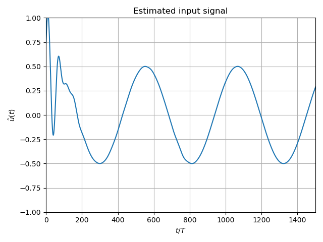
Estimating the input
Fortunately, we used the same analog system and digital controls as in this example so
174 stop_after_number_of_iterations = 1 << 17
175 u_hat = np.zeros(stop_after_number_of_iterations)
176 K1 = 1 << 10
177 K2 = 1 << 11
178 digital_estimator = cbadc.digital_estimator.DigitalEstimator(
179     analog_system, digital_control,
180     eta2,
181     K1,
182     K2,
183     stop_after_number_of_iterations=stop_after_number_of_iterations
184 )
185 # Set control signal iterator
186 digital_estimator(control_signal_sequences)
187 for index, u_hat_temp in enumerate(digital_estimator):
188     u_hat[index] = u_hat_temp
189
190 t = np.arange(u_hat.size)
191 plt.plot(t, u_hat)
192 plt.xlabel('$t / T$')
193 plt.ylabel('$\hat{u}(t)$')
194 plt.title("Estimated input signal")
195 plt.grid()
196 plt.xlim((0, 1500))
197 plt.ylim((-1, 1))
198 plt.tight_layout()
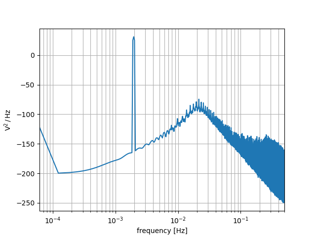
Plotting the PSD
As is typical for delta-sigma modulators, we often visualize the performance of the estimate by plotting the power spectral density (PSD).
207 f, psd = cbadc.utilities.compute_power_spectral_density(u_hat[K2:])
208 plt.figure()
209 plt.semilogx(f, 10 * np.log10(psd))
210 plt.xlabel('frequency [Hz]')
211 plt.ylabel('$ \mathrm{V}^2 \, / \, \mathrm{Hz}$')
212 plt.xlim((f[1], f[-1]))
213 plt.grid(which='both')
Total running time of the script: ( 0 minutes 14.936 seconds)