Simulating a Control-Bounded ADC

This example shows how to simulate the interactions between an analog system and a digital control while the former is excited by an analog signal.

import matplotlib.pyplot as plt
import cbadc
import numpy as np

The Analog System

First, we have to decide on an analog system. For this tutorial, we will commit to a chain-of-integrators ADC, see cbadc.analog_system.ChainOfIntegrators, as our analog system.

# We fix the number of analog states.
N = 6
# Set the amplification factor.
beta = 6250.
rho = - 1e-2
kappa = - 1.0
# In this example, each nodes amplification and local feedback will be set
# identically.
betaVec = beta * np.ones(N)
rhoVec = betaVec * rho
kappaVec = kappa * beta * np.eye(N)

# Instantiate a chain-of-integrators analog system.
analog_system = cbadc.analog_system.ChainOfIntegrators(betaVec, rhoVec, kappaVec)
# print the analog system such that we can very it being correctly initalized.
print(analog_system)

Out:

The analog system is parameterized as:
A =
[[ -62.5    0.     0.     0.     0.     0. ]
 [6250.   -62.5    0.     0.     0.     0. ]
 [   0.  6250.   -62.5    0.     0.     0. ]
 [   0.     0.  6250.   -62.5    0.     0. ]
 [   0.     0.     0.  6250.   -62.5    0. ]
 [   0.     0.     0.     0.  6250.   -62.5]],
B =
[[6250.]
 [   0.]
 [   0.]
 [   0.]
 [   0.]
 [   0.]],
CT =
[[1. 0. 0. 0. 0. 0.]
 [0. 1. 0. 0. 0. 0.]
 [0. 0. 1. 0. 0. 0.]
 [0. 0. 0. 1. 0. 0.]
 [0. 0. 0. 0. 1. 0.]
 [0. 0. 0. 0. 0. 1.]],
Gamma =
[[-6250.    -0.    -0.    -0.    -0.    -0.]
 [   -0. -6250.    -0.    -0.    -0.    -0.]
 [   -0.    -0. -6250.    -0.    -0.    -0.]
 [   -0.    -0.    -0. -6250.    -0.    -0.]
 [   -0.    -0.    -0.    -0. -6250.    -0.]
 [   -0.    -0.    -0.    -0.    -0. -6250.]],
Gamma_tildeT =
[[1. 0. 0. 0. 0. 0.]
 [0. 1. 0. 0. 0. 0.]
 [0. 0. 1. 0. 0. 0.]
 [0. 0. 0. 1. 0. 0.]
 [0. 0. 0. 0. 1. 0.]
 [0. 0. 0. 0. 0. 1.]], and D=[[0.]
 [0.]
 [0.]
 [0.]
 [0.]
 [0.]]

The Digital Control

In addition to the analog system, our simulation will require us to specify a digital control. For this tutorial, we will use cbadc.digital_control.DigitalControl.

# Set the time period which determines how often the digital control updates.
T = 1.0/(2 * beta)
# Set the number of digital controls to be same as analog states.
M = N
# Initialize the digital control.
digital_control = cbadc.digital_control.DigitalControl(T, M)
# print the digital control to verify proper initialization.
print(digital_control)

Out:

The Digital Control is parameterized as:
T = 8e-05,
M = 6, and next update at
t = 8e-05

The Analog Signal

The final and third component of the simulation is an analog signal. For this tutorial, we will choose a cbadc.analog_signal.Sinusodial. Again, this is one of several possible choices.

# Set the peak amplitude.
amplitude = 0.5
# Choose the sinusodial frequency via an oversampling ratio (OSR).
OSR = 1 << 9
frequency = 1.0 / (T * OSR)

# We also specify a phase an offset these are hovewer optional.
phase = np.pi / 3
offset = 0.0

# Instantiate the analog signal
analog_signal = cbadc.analog_signal.Sinusodial(amplitude, frequency, phase, offset)
# print to ensure correct parametrization.
print(analog_signal)

Out:

Sinusodial parameterized as:
amplitude = 0.5,

        frequency = 24.414062499999996,
phase = 1.0471975511965976,
        and
offset = 0.0

Simulating

Next, we set up the simulator. Here we use the cbadc.simulator.StateSpaceSimulator for simulating the involved differential equations as outlined in cbadc.analog_system.AnalogSystem.

# Simulate for 2^18 control cycles.
end_time = T * (1 << 18)

# Instantiate the simulator.
simulator = cbadc.simulator.StateSpaceSimulator(analog_system, digital_control, [
                                analog_signal], t_stop=end_time)
# Depending on your analog system the step above might take some time to
# compute as it involves precomputing solutions to initial value problems.

# Let's print the first 20 control decisions.
index = 0
for s in simulator:
    if (index > 19):
        break
    print(f"step:{index} -> s:{np.array(s)}")
    index += 1

# To verify the simulation parametrization we can
print(simulator)

Out:

step:0 -> s:[0 0 0 0 0 0]
step:1 -> s:[ True  True  True  True  True  True]
step:2 -> s:[False False False False False False]
step:3 -> s:[ True  True False False False False]
step:4 -> s:[ True False  True  True  True  True]
step:5 -> s:[ True  True  True False False False]
step:6 -> s:[False  True False  True  True False]
step:7 -> s:[ True False  True False False  True]
step:8 -> s:[ True  True False  True  True False]
step:9 -> s:[False False  True False False  True]
step:10 -> s:[ True  True False  True  True  True]
step:11 -> s:[ True  True  True  True  True False]
step:12 -> s:[ True  True  True False False  True]
step:13 -> s:[False False False  True  True False]
step:14 -> s:[ True  True  True False False False]
step:15 -> s:[ True  True False  True  True  True]
step:16 -> s:[ True False  True False False False]
step:17 -> s:[False  True False  True  True  True]
step:18 -> s:[ True False  True False False False]
step:19 -> s:[ True  True False  True  True  True]
t = 0.00168, (current simulator time)
Ts = 8e-05,
t_stop = 20.97152,
rtol = 1e-12,
atol = 1e-12, and
max_step = 0.0008

Tracking the Analog State Vector

Clearly the output type of the generator simulator above is the sequence of control signals s[k]. Sometimes we are interested in also monitoring the internal states of analog system during simulation.

To this end we use the cbadc.simulator.StateSpaceSimulator.state_vector() and an cbadc.simulator.extended_simulation_result().

Note that the cbadc.simulator.extended_simulation_result() is defined like this

def extended_simulation_result(simulator):
    for control_signal in simulator:
        analog_state = simulator.state_vector()
        yield {
            'control_signal': np.array(control_signal),
            'analog_state': np.array(analog_state)
        }

So, in essence, we are creating a new generator from the old with an extended output.

Note

The convenience function extended_simulation_result is one of many such convenience functions found in the cbadc.simulator module.

We can achieve this by appending yet another generator to the control signal stream as:

# Repeating the steps above we now get for the following
# ten control cycles.

ext_simulator = cbadc.simulator.extended_simulation_result(simulator)
for res in ext_simulator:
    if (index > 29):
        break
    print(
        f"step:{index} -> s:{res['control_signal']}, x:{res['analog_state']}")
    index += 1

Out:

step:20 -> s:[False False False  True  True  True], x:[ 0.54823676  0.11670772  0.06484886 -0.46198389 -0.49102059 -0.40805816]
step:21 -> s:[ True  True  True False False False], x:[ 0.28852725 -0.17409673 -0.44326189 -0.04946166 -0.10665263 -0.06475268]
step:22 -> s:[ True False False False False False], x:[0.03084446 0.4050305  0.12088599 0.35734476 0.45783109 0.51372668]
step:23 -> s:[ True  True  True  True  True  True], x:[-0.22485823 -0.14425853 -0.30835322 -0.17870188  0.01002193  0.13999125]
step:24 -> s:[False False False False  True  True], x:[ 0.51887684  0.42881669  0.24768117  0.29413072 -0.47129112 -0.48446692]
step:25 -> s:[ True  True  True  True False False], x:[ 0.2620199   0.12253093 -0.10960284 -0.16543741  0.0691172  -0.07384136]
step:26 -> s:[ True  True False False  True False], x:[ 0.00702877 -0.30986756  0.34809793  0.40279176 -0.38008514  0.33569678]
step:27 -> s:[ True False  True  True False  True], x:[-0.24614276  0.13067341 -0.19163271 -0.06832894  0.21496668 -0.19582836]
step:28 -> s:[False  True False False  True False], x:[ 0.4999634  -0.30514404  0.24888015  0.45427751 -0.19748233  0.2971895 ]
step:29 -> s:[ True False  True  True False  True], x:[ 0.24531795  0.38086046 -0.2266544  -0.05565045  0.41130859 -0.13881065]

Saving to File

In general, simulating the analog system and digital control interaction is a computationally much more intense procedure compared to the digital estimation step. This is one reason, and there are more, why you would want to store the intermediate control signal sequence to a file.

For this purpose use the cbadc.utilities.control_signal_2_byte_stream() and cbadc.utilities.write_byte_stream_to_file() functions.

# Instantiate a new simulator and control.
simulator = cbadc.simulator.StateSpaceSimulator(analog_system, digital_control, [
                                analog_signal], t_stop=end_time)

# Construct byte stream.
byte_stream = cbadc.utilities.control_signal_2_byte_stream(simulator, M)


def print_next_10_bytes(stream):
    global index
    for byte in stream:
        if (index < 40):
            print(f"{index} -> {byte}")
            index += 1
        yield byte


cbadc.utilities.write_byte_stream_to_file("sinusodial_simulation.adcs",
                          print_next_10_bytes(byte_stream))

Out:

30 -> b'\x13'
31 -> b'\x13'
32 -> b'\x13'
33 -> b'\x13'
34 -> b'\x13'
35 -> b'\x13'
36 -> b'\x13'
37 -> b'\x13'
38 -> b'\x13'
39 -> b'\x13'

Evaluating the Analog State Vector in Between Control Signal Samples

If we wish to simulate the analog state vector trajectory between control updates, this can be achieved using the Ts parameter of the cbadc.simulator.StateSpaceSimulator. Technically you can scale \(T_s = T / \alpha\) for any positive number \(\alpha\). For such a scaling, the simulator will generate \(\alpha\) more control signals per unit of time. However, digital control is still restricted to only update the control signals at multiples of \(T\).

# Set sampling time three orders of magnitude smaller than the control period
Ts = T / 1000.0

# Simulate for 10000 control cycles.
size = 15000
end_time = size * Ts

# Initialize a new digital control.
new_digital_control = cbadc.digital_control.DigitalControl(T, M)

# Instantiate a new simulator with a sampling time.
simulator = cbadc.simulator.StateSpaceSimulator(analog_system, new_digital_control, [
                                analog_signal], t_stop=end_time, Ts=Ts)

# Create data containers to hold the resulting data.
time_vector = np.arange(size) * Ts / T
states = np.zeros((N, size))
control_signals = np.zeros((M, size), dtype=np.int8)

# Iterate through and store states and control_signals.
for index, res in enumerate(cbadc.simulator.extended_simulation_result(simulator)):
    states[:, index] = res['analog_state']
    control_signals[:, index] = res['control_signal']

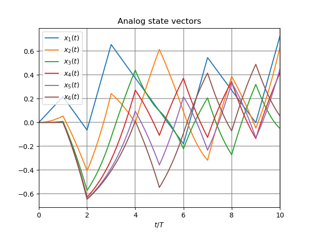
# Plot all analog state evolutions.
plt.figure()
plt.title("Analog state vectors")
for index in range(N):
    plt.plot(time_vector, states[index, :], label=f"$x_{index + 1}(t)$")
plt.grid(b=True, which='major', color='gray', alpha=0.6, lw=1.5)
plt.xlabel('$t/T$')
plt.xlim((0, 10))
plt.legend()

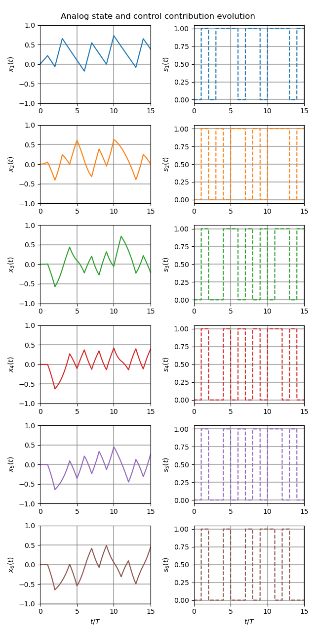
# reset figure size and plot individual results.
plt.rcParams['figure.figsize'] = [6.40, 6.40 * 2]
fig, ax = plt.subplots(N, 2)
for index in range(N):
    color = next(ax[0, 0]._get_lines.prop_cycler)['color']
    ax[index, 0].grid(b=True, which='major', color='gray', alpha=0.6, lw=1.5)
    ax[index, 1].grid(b=True, which='major', color='gray', alpha=0.6, lw=1.5)
    ax[index, 0].plot(time_vector, states[index, :], color=color)
    ax[index, 1].plot(time_vector, control_signals[index, :],
                      '--', color=color)
    ax[index, 0].set_ylabel(f"$x_{index + 1}(t)$")
    ax[index, 1].set_ylabel(f"$s_{index + 1}(t)$")
    ax[index, 0].set_xlim((0, 15))
    ax[index, 1].set_xlim((0, 15))
    ax[index, 0].set_ylim((-1, 1))
fig.suptitle("Analog state and control contribution evolution")
ax[-1, 0].set_xlabel("$t / T$")
ax[-1, 1].set_xlabel("$t / T$")
fig.tight_layout()

• 
• 

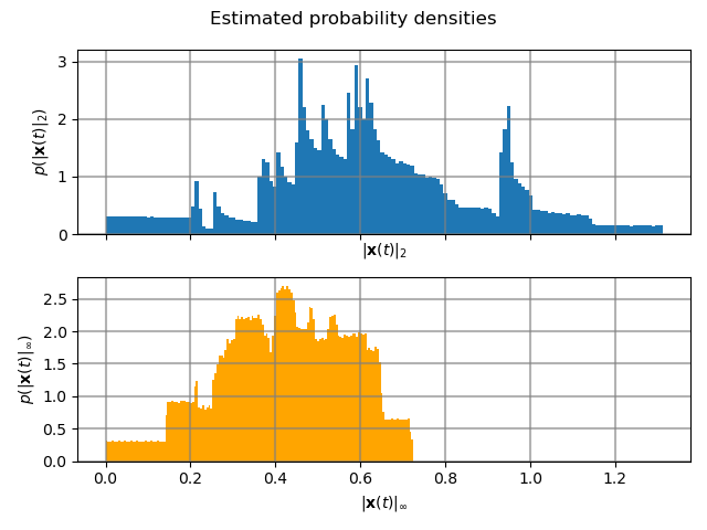
Analog State Statistics

As in the previous section, visualizing the analog state trajectory is a good way of identifying problems and possible errors. Another way of making sure that the analog states remain bounded is to estimate their corresponding densities (assuming i.i.d samples).

# Compute L_2 norm of analog state vector.
L_2_norm = np.linalg.norm(states, ord=2, axis=0)
# Similarly, compute L_infty (largest absolute value) of the analog state
# vector.
L_infty_norm = np.linalg.norm(states, ord=np.inf, axis=0)

# Estimate and plot densities using matplotlib tools.
bins = 150
plt.rcParams['figure.figsize'] = [6.40, 4.80]
fig, ax = plt.subplots(2, sharex=True)
ax[0].grid(b=True, which='major', color='gray', alpha=0.6, lw=1.5)
ax[1].grid(b=True, which='major', color='gray', alpha=0.6, lw=1.5)
ax[0].hist(L_2_norm, bins=bins, density=True)
ax[1].hist(L_infty_norm, bins=bins, density=True, color="orange")
plt.suptitle("Estimated probability densities")
ax[0].set_xlabel("$\|\mathbf{x}(t)\|_2$")
ax[1].set_xlabel("$\|\mathbf{x}(t)\|_\infty$")
ax[0].set_ylabel("$p ( \| \mathbf{x}(t) \|_2 ) $")
ax[1].set_ylabel("$p ( \| \mathbf{x}(t) \|_\infty )$")
fig.tight_layout()