Note
Click here to download the full example code
Compare Estimators
In this tutorial we investigate different estimator implementation techniques and compare their performance.
 8 import timeit
 9 import matplotlib.pyplot as plt
10 import numpy as np
11 import cbadc
Analog System
We will commit to a leap-frog control-bounded analog system throughtout this tutorial.
20 # Determine system parameters
21 N = 6
22 M = N
23 beta = 6250
24 # Set control period
25 T = 1.0 / (2.0 * beta)
26 # Adjust the feedback to achieve a bandwidth corresponding to OSR.
27 OSR = 128
28 omega_3dB = 2 * np.pi / (T * OSR)
29
30 # Instantiate analog system.
31 beta_vec = beta * np.ones(N)
32 rho_vec = - omega_3dB ** 2 / beta * np.ones(N)
33 Gamma = np.diag(-beta_vec)
34 analog_system = cbadc.analog_system.LeapFrog(beta_vec, rho_vec, Gamma)
35
36 print(analog_system, "\n")
Out:
The analog system is parameterized as:
A =
[[ -60.23928467  -60.23928467    0.            0.            0.
     0.        ]
 [6250.            0.          -60.23928467    0.            0.
     0.        ]
 [   0.         6250.            0.          -60.23928467    0.
     0.        ]
 [   0.            0.         6250.            0.          -60.23928467
     0.        ]
 [   0.            0.            0.         6250.            0.
   -60.23928467]
 [   0.            0.            0.            0.         6250.
     0.        ]],
B =
[[6250.]
 [   0.]
 [   0.]
 [   0.]
 [   0.]
 [   0.]],
CT =
[[1. 0. 0. 0. 0. 0.]
 [0. 1. 0. 0. 0. 0.]
 [0. 0. 1. 0. 0. 0.]
 [0. 0. 0. 1. 0. 0.]
 [0. 0. 0. 0. 1. 0.]
 [0. 0. 0. 0. 0. 1.]],
Gamma =
[[-6250.     0.     0.     0.     0.     0.]
 [    0. -6250.     0.     0.     0.     0.]
 [    0.     0. -6250.     0.     0.     0.]
 [    0.     0.     0. -6250.     0.     0.]
 [    0.     0.     0.     0. -6250.     0.]
 [    0.     0.     0.     0.     0. -6250.]],
Gamma_tildeT =
[[ 1. -0. -0. -0. -0. -0.]
 [-0.  1. -0. -0. -0. -0.]
 [-0. -0.  1. -0. -0. -0.]
 [-0. -0. -0.  1. -0. -0.]
 [-0. -0. -0. -0.  1. -0.]
 [-0. -0. -0. -0. -0.  1.]], and D=[[0.]
 [0.]
 [0.]
 [0.]
 [0.]
 [0.]]
Analog Signal
We will also need an analog signal for conversion. In this tutorial we will use a Sinusodial signal.
45 # Set the peak amplitude.
46 amplitude = 1.0
47 # Choose the sinusodial frequency via an oversampling ratio (OSR).
48 frequency = 1.0 / (T * OSR * (1 << 0))
49
50 # We also specify a phase an offset these are hovewer optional.
51 phase = 0.0
52 offset = 0.0
53
54 # Instantiate the analog signal
55 analog_signal = cbadc.analog_signal.Sinusodial(amplitude, frequency, phase, offset)
56
57 print(analog_signal)
Out:
Sinusodial parameterized as:
amplitude = 1.0,

        frequency = 97.65624999999999,
phase = 0.0,
        and
offset = 0.0
Simulating
Each estimator will require an independent stream of control signals. Therefore, we will next instantiate several digital controls and simulators.
 67 # Set simulation precision parameters
 68 atol = 1e-6
 69 rtol = 1e-12
 70 max_step = T / 10.
 71
 72 # Instantiate digital controls. We will need four of them as we will compare
 73 # four different estimators.
 74 digital_control1 = cbadc.digital_control.DigitalControl(T, M)
 75 digital_control2 = cbadc.digital_control.DigitalControl(T, M)
 76 digital_control3 = cbadc.digital_control.DigitalControl(T, M)
 77 digital_control4 = cbadc.digital_control.DigitalControl(T, M)
 78 print(digital_control1)
 79
 80 # Instantiate simulators.
 81 simulator1 = cbadc.simulator.StateSpaceSimulator(
 82     analog_system,
 83     digital_control1,
 84     [analog_signal],
 85     atol=atol,
 86     rtol=rtol,
 87     max_step=max_step
 88 )
 89 simulator2 = cbadc.simulator.StateSpaceSimulator(
 90     analog_system,
 91     digital_control2,
 92     [analog_signal],
 93     atol=atol,
 94     rtol=rtol,
 95     max_step=max_step
 96 )
 97 simulator3 = cbadc.simulator.StateSpaceSimulator(
 98     analog_system,
 99     digital_control3,
100     [analog_signal],
101     atol=atol,
102     rtol=rtol,
103     max_step=max_step
104 )
105 simulator4 = cbadc.simulator.StateSpaceSimulator(
106     analog_system,
107     digital_control4,
108     [analog_signal],
109     atol=atol,
110     rtol=rtol,
111     max_step=max_step
112 )
113 print(simulator1)
Out:
The Digital Control is parameterized as:
T = 8e-05,
M = 6, and next update at
t = 8e-05
t = 0.0, (current simulator time)
Ts = 8e-05,
t_stop = inf,
rtol = 1e-12,
atol = 1e-06, and
max_step = 8.000000000000001e-06
Default, Quadratic Complexity, Estimator
Next we instantiate the quadratic and default estimator
cbadc.digital_estimator.DigitalEstimator. Note that during its
construction, the corresponding filter coefficients of the system will be
computed. Therefore, this procedure could be computationally intense for a
analog system with a large analog state order or equivalently for large
number of independent digital controls.
126 # Set the bandwidth of the estimator
127 G_at_omega = np.linalg.norm(
128     analog_system.transfer_function_matrix(np.array([omega_3dB])))
129 eta2 = G_at_omega**2
130 print(f"eta2 = {eta2}, {10 * np.log10(eta2)} [dB]")
131
132 # Set the batch size
133 K1 = 1 << 14
134 K2 = 1 << 14
135
136 # Instantiate the digital estimator (this is where the filter coefficients are
137 # computed).
138 digital_estimator_batch = cbadc.digital_estimator.DigitalEstimator(
139     analog_system, digital_control1, eta2, K1, K2)
140 digital_estimator_batch(simulator1)
141
142 print(digital_estimator_batch, "\n")
Out:
eta2 = 1259410956005.0083, 121.00167467044352 [dB]
Digital estimator is parameterized as

eta2 = 1259410956005.01, 121 [dB],

Ts = 8e-05,
K1 = 16384,
K2 = 16384,

and
number_of_iterations = 9223372036854775808

Resulting in the filter coefficients
Af =
[[ 9.93992011e-01 -4.80368682e-03  1.15864448e-05 -1.85515926e-08
   1.63410461e-10 -7.50223347e-11]
 [ 4.98396397e-01  9.97593569e-01 -4.81334317e-03  1.16016953e-05
  -1.11135428e-08  1.65593448e-08]
 [ 1.24724256e-01  4.99398045e-01  9.97591782e-01 -4.81356428e-03
   1.13768870e-05  1.77374670e-07]
 [ 2.07981872e-02  1.24899305e-01  4.99395630e-01  9.97581755e-01
  -4.83705939e-03 -1.55238302e-05]
 [ 2.60019384e-03  2.08166882e-02  1.24867079e-01  4.99198307e-01
   9.96748934e-01 -6.25618007e-03]
 [ 2.57435177e-04  2.57297257e-03  2.05433050e-02  1.22849014e-01
   4.88154288e-01  9.59742079e-01]],

Ab =
[[ 1.00362260e+00  4.82689704e-03  1.16236702e-05  1.86786149e-08
   2.09634411e-10 -1.97644500e-10]
 [-5.00804522e-01  9.97589700e-01  4.81334112e-03  1.15948304e-05
   2.15247962e-08  1.18496522e-08]
 [ 1.25125657e-01 -4.99397548e-01  9.97591713e-01  4.81382778e-03
   1.07124083e-05  6.90493753e-07]
 [-2.08483433e-02  1.24899069e-01 -4.99394396e-01  9.97575580e-01
   4.85758001e-03 -5.16212805e-05]
 [ 2.60500526e-03 -2.08147709e-02  1.24852463e-01 -4.99111003e-01
   9.96381087e-01  7.05497103e-03]
 [-2.56748688e-04  2.56174243e-03 -2.04480404e-02  1.22206039e-01
  -4.84970386e-01  9.50489454e-01]],

Bf =
[[-4.98596881e-01  1.20236964e-03 -1.93231278e-06  2.31454333e-09
  -3.97667688e-11  1.54595883e-11]
 [-1.24749327e-01 -4.99598767e-01  1.20406083e-03 -1.93395884e-06
   8.49726057e-10 -4.20727403e-09]
 [-2.08007368e-02 -1.24924740e-01 -4.99598530e-01  1.20411261e-03
  -1.87040237e-06 -4.10128618e-08]
 [-2.60081858e-03 -2.08232546e-02 -1.24924376e-01 -4.99596513e-01
   1.20951927e-03  5.19835323e-06]
 [-2.60096754e-04 -2.60270056e-03 -2.08191933e-02 -1.24892521e-01
  -4.99417729e-01  1.57454839e-03]
 [-2.14752207e-05 -2.57642154e-04 -2.57316206e-03 -2.05457499e-02
  -1.22909157e-01 -4.89999233e-01]],

Bb =
[[ 5.01005490e-01  1.20623894e-03  1.93696031e-06  2.34138942e-09
   4.37598487e-11 -5.22665975e-11]
 [-1.25150778e-01  4.99598283e-01  1.20406088e-03  1.93243952e-06
   3.44418666e-09  2.83912996e-09]
 [ 2.08509199e-02 -1.24924690e-01  4.99598518e-01  1.20416489e-03
   1.72011597e-06  1.85227740e-07]
 [-2.60583470e-03  2.08232276e-02 -1.24924193e-01  4.99595398e-01
   1.21392827e-03 -1.44616071e-05]
 [ 2.60496116e-04 -2.60249443e-03  2.08172912e-02 -1.24878394e-01
   4.99342305e-01  1.77775324e-03]
 [-2.14127285e-05  2.56542055e-04 -2.56194098e-03  2.04515506e-02
  -1.22306845e-01  4.87667659e-01]],

and WT =
[[ 3.72587867e-02  3.59110826e-04 -3.04746438e-05 -2.93722946e-07
   3.97693792e-08  3.78364448e-10]].
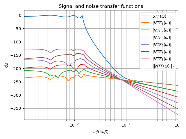
Visualize Estimator’s Transfer Function (Same for Both)
150 # Logspace frequencies
151 frequencies = np.logspace(-3, 0, 100)
152 omega = 4 * np.pi * beta * frequencies
153
154 # Compute NTF
155 ntf = digital_estimator_batch.noise_transfer_function(omega)
156 ntf_dB = 20 * np.log10(np.abs(ntf))
157
158 # Compute STF
159 stf = digital_estimator_batch.signal_transfer_function(omega)
160 stf_dB = 20 * np.log10(np.abs(stf.flatten()))
161
162 # Signal attenuation at the input signal frequency
163 stf_at_omega = digital_estimator_batch.signal_transfer_function(
164     np.array([2 * np.pi * frequency]))[0]
165
166 # Plot
167 plt.figure()
168 plt.semilogx(frequencies, stf_dB, label='$STF(\omega)$')
169 for n in range(N):
170     plt.semilogx(frequencies, ntf_dB[0, n, :], label=f"$|NTF_{n+1}(\omega)|$")
171 plt.semilogx(frequencies, 20 * np.log10(np.linalg.norm(
172     ntf[0, :, :], axis=0)), '--', label="$ || NTF(\omega) ||_2 $")
173
174 # Add labels and legends to figure
175 plt.legend()
176 plt.grid(which='both')
177 plt.title("Signal and noise transfer functions")
178 plt.xlabel("$\omega / (4 \pi \\beta ) $")
179 plt.ylabel("dB")
180 plt.xlim((frequencies[1], frequencies[-1]))
181 plt.gcf().tight_layout()
FIR Filter Estimator
Similarly as for the previous estimator the
cbadc.digital_estimator.FIRFilter is initalized. Additionally,
we visualize the decay of the \(\|\cdot\|_2\) norm of the corresponding
filter coefficients. This is an aid to determine if the lookahead and
lookback sizes L1 and L2 are set sufficiently large.
193 # Determine lookback
194 L1 = K2
195 # Determine lookahead
196 L2 = K2
197 digital_estimator_fir = cbadc.digital_estimator.FIRFilter(
198     analog_system, digital_control2, eta2, L1, L2)
199
200 print(digital_estimator_fir, "\n")
201
202 digital_estimator_fir(simulator2)
203
204 # Next visualize the decay of the resulting filter coefficients.
205 h_index = np.arange(-L1, L2)
206
207 impulse_response = np.abs(np.array(digital_estimator_fir.h[0, :, :])) ** 2
208 impulse_response_dB = 10 * np.log10(impulse_response)
209
210 fig, ax = plt.subplots(2)
211 for index in range(N):
212     ax[0].plot(h_index, impulse_response[:, index],
213                label=f"$h_{index + 1}[k]$")
214     ax[1].plot(h_index, impulse_response_dB[:, index],
215                label=f"$h_{index + 1}[k]$")
216 ax[0].legend()
217 fig.suptitle(f"For $\eta^2 = {10 * np.log10(eta2)}$ [dB]")
218 ax[1].set_xlabel("filter taps k")
219 ax[0].set_ylabel("$| h_\ell [k]|^2_2$")
220 ax[1].set_ylabel("$| h_\ell [k]|^2_2$ [dB]")
221 ax[0].set_xlim((-50, 50))
222 ax[0].grid(which='both')
223 ax[1].set_xlim((-50, 500))
224 ax[1].set_ylim((-200, 0))
225 ax[1].grid(which='both')
![For $\eta^2 = 121.00167467044352$ [dB]](../../_images/sphx_glr_plot_a_compare_estimator_002.png)
Out:
FIR estimator is parameterized as
eta2 = 1259410956005.01, 121 [dB],
Ts = 8e-05,
K1 = 16384,
K2 = 16384,
and
number_of_iterations = 9223372036854775808.
Resulting in the filter coefficients
h =
[[[-8.98888895e-23  3.86415093e-22  1.78156003e-24 -4.79446969e-24
    7.27065590e-26  2.27668499e-26]
  [-2.83409887e-22  3.83559844e-22  6.03912514e-24 -4.80331076e-24
    3.78726684e-26  2.38832692e-26]
  [-4.75669187e-22  3.77650777e-22  1.02704857e-23 -4.77413572e-24
    2.56155334e-27  2.48161161e-26]
  ...
  [-4.75669905e-22 -3.86819971e-22  2.90231506e-24  4.90109883e-24
    9.58043250e-26 -2.39133320e-26]
  [-2.83410643e-22 -3.89022950e-22 -1.40723095e-24  4.84795441e-24
    1.30885020e-25 -2.23089598e-26]
  [-8.98896788e-23 -3.88147790e-22 -5.68388014e-24  4.75685837e-24
    1.64756362e-25 -2.05368240e-26]]].
IIR Filter Estimator
The IIR filter is closely related to the FIR filter with the exception
of an moving average computation.
See cbadc.digital_estimator.IIRFilter for more information.
236 # Determine lookahead
237 L2 = K2
238
239 digital_estimator_iir = cbadc.digital_estimator.IIRFilter(
240     analog_system, digital_control3, eta2, L2)
241
242 print(digital_estimator_iir, "\n")
243
244 digital_estimator_iir(simulator3)
Out:
IIR estimator is parameterized as
eta2 = 1259410956005.01, 121 [dB],
Ts = 8e-05,
K2 = 16384,
and
number_of_iterations = 9223372036854775808.
Resulting in the filter coefficients
Af =
[[ 9.93992011e-01 -4.80368682e-03  1.15864448e-05 -1.85515926e-08
   1.63410461e-10 -7.50223347e-11]
 [ 4.98396397e-01  9.97593569e-01 -4.81334317e-03  1.16016953e-05
  -1.11135428e-08  1.65593448e-08]
 [ 1.24724256e-01  4.99398045e-01  9.97591782e-01 -4.81356428e-03
   1.13768870e-05  1.77374670e-07]
 [ 2.07981872e-02  1.24899305e-01  4.99395630e-01  9.97581755e-01
  -4.83705939e-03 -1.55238302e-05]
 [ 2.60019384e-03  2.08166882e-02  1.24867079e-01  4.99198307e-01
   9.96748934e-01 -6.25618007e-03]
 [ 2.57435177e-04  2.57297257e-03  2.05433050e-02  1.22849014e-01
   4.88154288e-01  9.59742079e-01]],
Bf =
[[-4.98596881e-01  1.20236964e-03 -1.93231278e-06  2.31454333e-09
  -3.97667688e-11  1.54595883e-11]
 [-1.24749327e-01 -4.99598767e-01  1.20406083e-03 -1.93395884e-06
   8.49726057e-10 -4.20727403e-09]
 [-2.08007368e-02 -1.24924740e-01 -4.99598530e-01  1.20411261e-03
  -1.87040237e-06 -4.10128618e-08]
 [-2.60081858e-03 -2.08232546e-02 -1.24924376e-01 -4.99596513e-01
   1.20951927e-03  5.19835323e-06]
 [-2.60096754e-04 -2.60270056e-03 -2.08191933e-02 -1.24892521e-01
  -4.99417729e-01  1.57454839e-03]
 [-2.14752207e-05 -2.57642154e-04 -2.57316206e-03 -2.05457499e-02
  -1.22909157e-01 -4.89999233e-01]],WT =
[[ 3.72587867e-02  3.59110826e-04 -3.04746438e-05 -2.93722946e-07
   3.97693792e-08  3.78364448e-10]],
 and h =
[[[ 1.86212790e-02  2.28154967e-04 -1.46830068e-05 -1.87616529e-07
    1.94061457e-08  2.52891376e-10]
  [ 1.85726421e-02  3.24796863e-04 -1.32368982e-05 -2.64504812e-07
    1.81534337e-08  3.75850026e-10]
  [ 1.84756128e-02  4.20239297e-04 -1.12914286e-05 -3.32485461e-07
    1.64896942e-08  4.90005466e-10]
  ...
  [-4.75669905e-22 -3.86819971e-22  2.90231506e-24  4.90109883e-24
    9.58043250e-26 -2.39133320e-26]
  [-2.83410643e-22 -3.89022950e-22 -1.40723095e-24  4.84795441e-24
    1.30885020e-25 -2.23089598e-26]
  [-8.98896788e-23 -3.88147790e-22 -5.68388014e-24  4.75685837e-24
    1.64756362e-25 -2.05368240e-26]]].
Parallel Estimator
Next we instantiate the parallel estimator
cbadc.digital_estimator.ParallelEstimator. The parallel estimator
resembles the default estimator but diagonalizes the filter coefficients
resulting in a more computationally more efficient filter that can be
parallelized into independent filter operations.
256 # Instantiate the digital estimator (this is where the filter coefficients are
257 # computed).
258 digital_estimator_parallel = cbadc.digital_estimator.ParallelEstimator(
259     analog_system, digital_control4, eta2, K1, K2)
260
261 digital_estimator_parallel(simulator4)
262 print(digital_estimator_parallel, "\n")
Out:
Parallel estimator is parameterized as
eta2 = 1259410956005.01, 121 [dB],
Ts = 8e-05,
K1 = 16384,
K2 = 16384,
and
number_of_iterations = 9223372036854775808
Resulting in the filter coefficients
f_a =
[0.99352853+0.08855482j 0.99352853-0.08855482j 0.99020742+0.06151822j
 0.99020742-0.06151822j 0.98788911+0.02199108j 0.98788911-0.02199108j],
b_a =
[[-1.38136935e+03+2.51506293e+03j  4.26841429e+02+2.82595564e+02j
   3.90945213e+01-5.02154026e+01j -4.61566859e+00-4.48169798e+00j
  -4.43374620e-01+3.13952416e-01j  9.36956969e-03+3.68208127e-02j]
 [-1.38136935e+03-2.51506293e+03j  4.26841429e+02-2.82595564e+02j
   3.90945213e+01+5.02154026e+01j -4.61566859e+00+4.48169798e+00j
  -4.43374620e-01-3.13952416e-01j  9.36956969e-03-3.68208127e-02j]
 [ 3.02676362e+03-8.51639570e+03j -9.79746501e+02-5.92495175e+02j
  -5.98609064e+01+3.01180862e+01j -6.65317488e+00+2.19446920e+00j
  -4.09920461e-01+1.15069267e+00j  7.27422100e-02+8.92621035e-02j]
 [ 3.02676362e+03+8.51639570e+03j -9.79746501e+02+5.92495175e+02j
  -5.98609064e+01-3.01180862e+01j -6.65317488e+00-2.19446920e+00j
  -4.09920461e-01-1.15069267e+00j  7.27422100e-02-8.92621035e-02j]
 [ 1.64587846e+03-1.36561516e+04j -5.52732368e+02-5.30916615e+02j
  -2.09658328e+01-1.19692787e+02j -1.11559461e+01-7.04141499e+00j
  -7.81738548e-01-8.25159236e-01j -1.63333052e-01-5.22025352e-02j]
 [ 1.64587846e+03+1.36561516e+04j -5.52732368e+02+5.30916615e+02j
  -2.09658328e+01+1.19692787e+02j -1.11559461e+01+7.04141499e+00j
  -7.81738548e-01+8.25159236e-01j -1.63333052e-01+5.22025352e-02j]],
f_b =
[[ 1.38153996e+03-2.51528946e+03j  4.53510548e+02+2.34143075e+02j
  -3.06136063e+01+5.52005619e+01j -5.28796590e+00-3.46613061e+00j
   3.47968904e-01-3.90570686e-01j  1.68823963e-02+3.00750056e-02j]
 [ 1.38153996e+03+2.51528946e+03j  4.53510548e+02-2.34143075e+02j
  -3.06136063e+01-5.52005619e+01j -5.28796590e+00+3.46613061e+00j
   3.47968904e-01+3.90570686e-01j  1.68823963e-02-3.00750056e-02j]
 [ 3.02777145e+03-8.51896570e+03j  1.03840481e+03+4.28469244e+02j
  -4.04251316e+01+3.99688739e+01j  5.68846326e+00-1.51947402e+00j
  -2.91086803e-01+1.11522405e+00j -7.93111153e-02-6.76031065e-02j]
 [ 3.02777145e+03+8.51896570e+03j  1.03840481e+03-4.28469244e+02j
  -4.04251316e+01-3.99688739e+01j  5.68846326e+00+1.51947402e+00j
  -2.91086803e-01-1.11522405e+00j -7.93111153e-02+6.76031065e-02j]
 [-1.64668442e+03+1.36624329e+04j -5.84727395e+02-2.67798132e+02j
   1.00094661e+01+1.12047350e+02j -1.08624178e+01-4.81058892e+00j
   5.69853789e-01+7.11277929e-01j -1.50265682e-01-3.75273959e-02j]
 [-1.64668442e+03-1.36624329e+04j -5.84727395e+02+2.67798132e+02j
   1.00094661e+01-1.12047350e+02j -1.08624178e+01+4.81058892e+00j
   5.69853789e-01-7.11277929e-01j -1.50265682e-01+3.75273959e-02j]],
b_b =
[[-1.38136935e+03+2.51506293e+03j  4.26841429e+02+2.82595564e+02j
   3.90945213e+01-5.02154026e+01j -4.61566859e+00-4.48169798e+00j
  -4.43374620e-01+3.13952416e-01j  9.36956969e-03+3.68208127e-02j]
 [-1.38136935e+03-2.51506293e+03j  4.26841429e+02-2.82595564e+02j
   3.90945213e+01+5.02154026e+01j -4.61566859e+00+4.48169798e+00j
  -4.43374620e-01-3.13952416e-01j  9.36956969e-03-3.68208127e-02j]
 [ 3.02676362e+03-8.51639570e+03j -9.79746501e+02-5.92495175e+02j
  -5.98609064e+01+3.01180862e+01j -6.65317488e+00+2.19446920e+00j
  -4.09920461e-01+1.15069267e+00j  7.27422100e-02+8.92621035e-02j]
 [ 3.02676362e+03+8.51639570e+03j -9.79746501e+02+5.92495175e+02j
  -5.98609064e+01-3.01180862e+01j -6.65317488e+00-2.19446920e+00j
  -4.09920461e-01-1.15069267e+00j  7.27422100e-02-8.92621035e-02j]
 [ 1.64587846e+03-1.36561516e+04j -5.52732368e+02-5.30916615e+02j
  -2.09658328e+01-1.19692787e+02j -1.11559461e+01-7.04141499e+00j
  -7.81738548e-01-8.25159236e-01j -1.63333052e-01-5.22025352e-02j]
 [ 1.64587846e+03+1.36561516e+04j -5.52732368e+02+5.30916615e+02j
  -2.09658328e+01+1.19692787e+02j -1.11559461e+01+7.04141499e+00j
  -7.81738548e-01+8.25159236e-01j -1.63333052e-01+5.22025352e-02j]],
f_w =
[[ 3.03885798e-07+2.89096208e-07j  3.03885798e-07-2.89096208e-07j
   1.85353652e-07+3.27557818e-07j  1.85353652e-07-3.27557818e-07j
  -6.07297807e-08-3.44886116e-07j -6.07297807e-08+3.44886116e-07j]],
and b_w =
[[-3.03911445e-07-2.89128776e-07j -3.03911445e-07+2.89128776e-07j
   1.85407011e-07+3.27659636e-07j  1.85407011e-07-3.27659636e-07j
   6.07565225e-08+3.45045111e-07j  6.07565225e-08-3.45045111e-07j]].
Estimating (Filtering)
Next we execute all simulation and estimation tasks by iterating over the estimators. Note that since no stop criteria is set for either the analog signal, the simulator, or the digital estimator this iteration could potentially continue until the default stop criteria of 2^63 iterations.
274 # Set simulation length
275 size = K2 << 4
276 u_hat_batch = np.zeros(size)
277 u_hat_fir = np.zeros(size)
278 u_hat_iir = np.zeros(size)
279 u_hat_parallel = np.zeros(size)
280 for index in range(size):
281     u_hat_batch[index] = next(digital_estimator_batch)
282     u_hat_fir[index] = next(digital_estimator_fir)
283     u_hat_iir[index] = next(digital_estimator_iir)
284     u_hat_parallel[index] = next(digital_estimator_parallel)
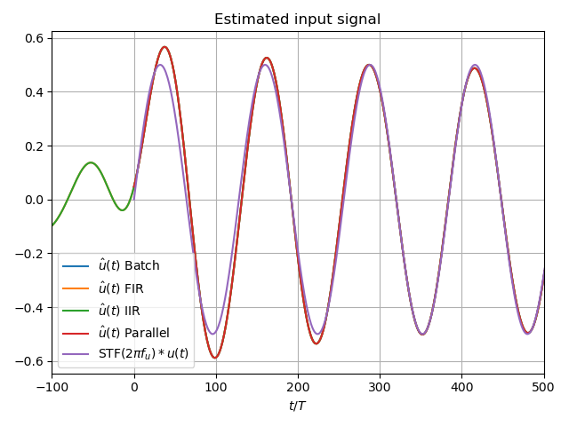
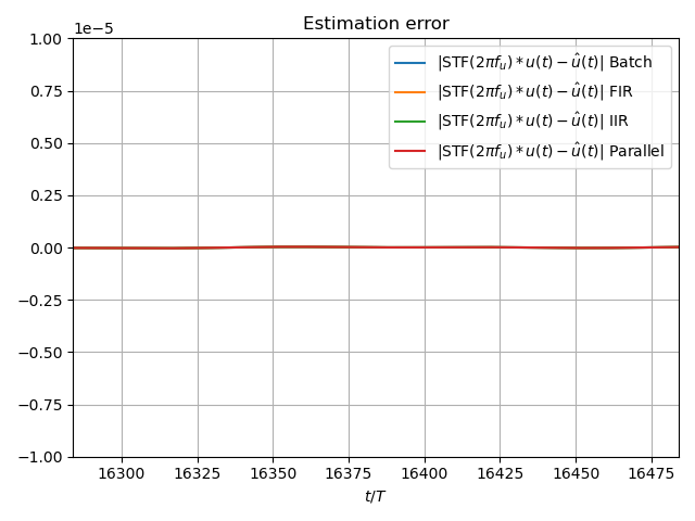
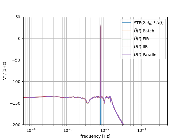
Visualizing Results
Finally, we summarize the comparision by visualizing the resulting estimate in both time and frequency domain.
293 t = np.arange(size)
294 # compensate the built in L1 delay of FIR filter.
295 t_fir = np.arange(-L1 + 1, size - L1 + 1)
296 t_iir = np.arange(-L1 + 1, size - L1 + 1)
297 u = np.zeros_like(u_hat_batch)
298 for index, tt in enumerate(t):
299 u[index] = analog_signal.evaluate(tt * T)
300 plt.plot(t, u_hat_batch, label="$\hat{u}(t)$ Batch")
301 plt.plot(t_fir, u_hat_fir, label="$\hat{u}(t)$ FIR")
302 plt.plot(t_iir, u_hat_iir, label="$\hat{u}(t)$ IIR")
303 plt.plot(t, u_hat_parallel, label="$\hat{u}(t)$ Parallel")
304 plt.plot(t, stf_at_omega * u, label="$\mathrm{STF}(2 \pi f_u) * u(t)$")
305 plt.xlabel('$t / T$')
306 plt.legend()
307 plt.title("Estimated input signal")
308 plt.grid(which='both')
309 plt.xlim((-100, 500))
310 plt.tight_layout()
311
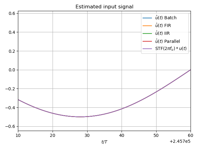
312 plt.figure()
313 plt.plot(t, u_hat_batch, label="$\hat{u}(t)$ Batch")
314 plt.plot(t_fir, u_hat_fir, label="$\hat{u}(t)$ FIR")
315 plt.plot(t_iir, u_hat_iir, label="$\hat{u}(t)$ IIR")
316 plt.plot(t, u_hat_parallel, label="$\hat{u}(t)$ Parallel")
317 plt.plot(t, stf_at_omega * u, label="$\mathrm{STF}(2 \pi f_u) * u(t)$")
318 plt.xlabel('$t / T$')
319 plt.legend()
320 plt.title("Estimated input signal")
321 plt.grid(which='both')
322 plt.xlim((t_fir[-1] - 50, t_fir[-1]))
323 plt.tight_layout()
324
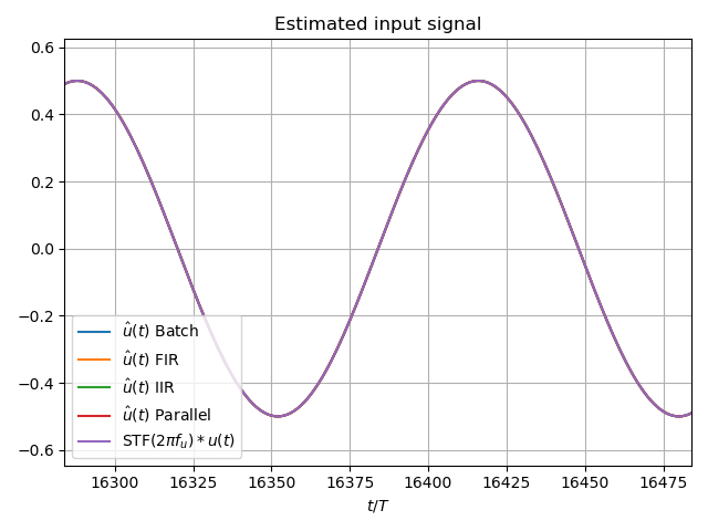
325 plt.figure()
326 plt.plot(t, u_hat_batch, label="$\hat{u}(t)$ Batch")
327 plt.plot(t_fir, u_hat_fir, label="$\hat{u}(t)$ FIR")
328 plt.plot(t_iir, u_hat_iir, label="$\hat{u}(t)$ IIR")
329 plt.plot(t, u_hat_parallel, label="$\hat{u}(t)$ Parallel")
330 plt.plot(t, stf_at_omega * u, label="$\mathrm{STF}(2 \pi f_u) * u(t)$")
331 plt.xlabel('$t / T$')
332 plt.legend()
333 plt.title("Estimated input signal")
334 plt.grid(which='both')
335 # plt.xlim((t_fir[0], t[-1]))
336 plt.xlim(((1 << 14) - 100, (1 << 14) + 100))
337 plt.tight_layout()
338
339 batch_error = stf_at_omega * u - u_hat_batch
340 fir_error = stf_at_omega * u[:(u.size - L1 + 1)] - u_hat_fir[(L1 - 1):]
341 iir_error = stf_at_omega * u[:(u.size - L1 + 1)] - u_hat_iir[(L1 - 1):]
342 parallel_error = stf_at_omega * u - u_hat_parallel
343 plt.figure()
344 plt.plot(t, batch_error,
345 label="$|\mathrm{STF}(2 \pi f_u) * u(t) - \hat{u}(t)|$ Batch")
346 plt.plot(t[:(u.size - L1 + 1)], fir_error,
347 label="$|\mathrm{STF}(2 \pi f_u) * u(t) - \hat{u}(t)|$ FIR")
348 plt.plot(t[:(u.size - L1 + 1)], iir_error,
349 label="$|\mathrm{STF}(2 \pi f_u) * u(t) - \hat{u}(t)|$ IIR")
350 plt.plot(t, parallel_error,
351 label="$|\mathrm{STF}(2 \pi f_u) * u(t) - \hat{u}(t)|$ Parallel")
352 plt.xlabel('$t / T$')
353 plt.xlim(((1 << 14) - 100, (1 << 14) + 100))
354 plt.ylim((-0.00001, 0.00001))
355 plt.legend()
356 plt.title("Estimation error")
357 plt.grid(which='both')
358 plt.tight_layout()
359
360
361 print(f"Average Batch Error: {np.linalg.norm(batch_error) / batch_error.size}")
362 print(f"Average FIR Error: {np.linalg.norm(fir_error) / fir_error.size}")
363 print(f"Average IIR Error: {np.linalg.norm(iir_error) / iir_error.size}")
364 print(
365 f"""Average Parallel Error: { np.linalg.norm(parallel_error)/
366 parallel_error.size}""")
367
368 plt.figure()
369 u_hat_batch_clipped = u_hat_batch[(K1 + K2):-K2]
370 u_hat_fir_clipped = u_hat_fir[(L1 + L2):]
371 u_hat_iir_clipped = u_hat_iir[(K1 + K2):-K2]
372 u_hat_parallel_clipped = u_hat_parallel[(K1 + K2):-K2]
373 u_clipped = stf_at_omega * u
374 f_batch, psd_batch = cbadc.utilities.compute_power_spectral_density(
375 u_hat_batch_clipped)
376 f_fir, psd_fir = cbadc.utilities.compute_power_spectral_density(
377 u_hat_fir_clipped)
378 f_iir, psd_iir = cbadc.utilities.compute_power_spectral_density(
379 u_hat_iir_clipped)
380 f_parallel, psd_parallel = cbadc.utilities.compute_power_spectral_density(
381 u_hat_parallel_clipped)
382 f_ref, psd_ref = cbadc.utilities.compute_power_spectral_density(u_clipped)
383 plt.semilogx(f_ref, 10 * np.log10(psd_ref),
384 label="$\mathrm{STF}(2 \pi f_u) * U(f)$")
385 plt.semilogx(f_batch, 10 * np.log10(psd_batch), label="$\hat{U}(f)$ Batch")
386 plt.semilogx(f_fir, 10 * np.log10(psd_fir), label="$\hat{U}(f)$ FIR")
387 plt.semilogx(f_iir, 10 * np.log10(psd_iir), label="$\hat{U}(f)$ IIR")
388 plt.semilogx(f_parallel, 10 * np.log10(psd_parallel),
389 label="$\hat{U}(f)$ Parallel")
390 plt.legend()
391 plt.ylim((-200, 50))
392 plt.xlim((f_fir[1], f_fir[-1]))
393 plt.xlabel('frequency [Hz]')
394 plt.ylabel('$ \mathrm{V}^2 \, / \, (1 \mathrm{Hz})$')
395 plt.grid(which='both')
396 plt.show()
Out:
Average Batch Error: 4.083356807183407e-06
Average FIR Error: 4.355562871483952e-06
Average IIR Error: 4.355562871483949e-06
Average Parallel Error: 4.083356808847717e-06
Compute Time
Compare the execution time of each estimator
406 def dummy_input_control_signal():
407     while True:
408         yield np.zeros(M, dtype=np.int8)
409
410
411 def iterate_number_of_times(iterator, number_of_times):
412     for _ in range(number_of_times):
413         _ = next(iterator)
414
415
416 digital_estimator_batch = cbadc.digital_estimator.DigitalEstimator(
417     analog_system,
418     digital_control1,
419     eta2,
420     K1,
421     K2)
422 digital_estimator_fir = cbadc.digital_estimator.FIRFilter(
423     analog_system,
424     digital_control2,
425     eta2,
426     L1,
427     L2)
428 digital_estimator_parallel = cbadc.digital_estimator.ParallelEstimator(
429     analog_system,
430     digital_control4,
431     eta2,
432     K1,
433     K2)
434 digital_estimator_iir = cbadc.digital_estimator.IIRFilter(
435     analog_system,
436     digital_control3,
437     eta2,
438     L2)
439
440 digital_estimator_batch(dummy_input_control_signal())
441 digital_estimator_fir(dummy_input_control_signal())
442 digital_estimator_parallel(dummy_input_control_signal())
443 digital_estimator_iir(dummy_input_control_signal())
444
445 length = 1 << 14
446 repetitions = 10
447
448 print("Digital Estimator:")
449 print(timeit.timeit(lambda: iterate_number_of_times(
450     digital_estimator_batch, length), number=repetitions), 'sec \n')
451
452 print("FIR Estimator:")
453 print(timeit.timeit(lambda: iterate_number_of_times(
454     digital_estimator_fir, length), number=repetitions), 'sec \n')
455
456 print("IIR Estimator:")
457 print(timeit.timeit(lambda: iterate_number_of_times(
458     digital_estimator_iir, length), number=repetitions), 'sec \n')
459
460 print("Parallel Estimator:")
461 print(timeit.timeit(lambda: iterate_number_of_times(
462     digital_estimator_parallel, length), number=repetitions), 'sec \n')
Out:
Digital Estimator:
5.485120426994399 sec

FIR Estimator:
37.11588862899225 sec

IIR Estimator:
36.34378033899702 sec

Parallel Estimator:
9.21785790399008 sec
Total running time of the script: ( 40 minutes 23.772 seconds)