Note
Click here to download the full example code
Downsampling
In this tutorial we demonstrate how to configure the digital estimator for downsampling.
 9 import scipy.signal
10 import numpy as np
11 import cbadc as cbc
12 import matplotlib.pyplot as plt
Setting up the Analog System and Digital Control
In this example, we assume that we have access to a control signal s[k] generated by the interactions of an analog system and digital control. Furthermore, we a chain-of-integrators converter with corresponding analog system and digital control.

28 # Setup analog system and digital control
29
30 # We fix the number of analog states.
31 N = 6
32 M = N
33 # Set the amplification factor.
34 beta = 6250.
35 rho = - 1e-2
36 kappa = - 1.0
37 # In this example, each nodes amplification and local feedback will be set
38 # identically.
39 betaVec = beta * np.ones(N)
40 rhoVec = betaVec * rho
41 kappaVec = kappa * beta * np.eye(N)
42
43 # Instantiate a chain-of-integrators analog system.
44 analog_system = cbc.analog_system.ChainOfIntegrators(betaVec, rhoVec, kappaVec)
45
46
47 T = 1/(2 * beta)
48 digital_control = cbc.digital_control.DigitalControl(T, M)
49
50
51 # Summarize the analog system, digital control, and digital estimator.
52 print(analog_system, "\n")
53 print(digital_control)
Out:
The analog system is parameterized as:
A =
[[ -62.5    0.     0.     0.     0.     0. ]
 [6250.   -62.5    0.     0.     0.     0. ]
 [   0.  6250.   -62.5    0.     0.     0. ]
 [   0.     0.  6250.   -62.5    0.     0. ]
 [   0.     0.     0.  6250.   -62.5    0. ]
 [   0.     0.     0.     0.  6250.   -62.5]],
B =
[[6250.]
 [   0.]
 [   0.]
 [   0.]
 [   0.]
 [   0.]],
CT =
[[1. 0. 0. 0. 0. 0.]
 [0. 1. 0. 0. 0. 0.]
 [0. 0. 1. 0. 0. 0.]
 [0. 0. 0. 1. 0. 0.]
 [0. 0. 0. 0. 1. 0.]
 [0. 0. 0. 0. 0. 1.]],
Gamma =
[[-6250.    -0.    -0.    -0.    -0.    -0.]
 [   -0. -6250.    -0.    -0.    -0.    -0.]
 [   -0.    -0. -6250.    -0.    -0.    -0.]
 [   -0.    -0.    -0. -6250.    -0.    -0.]
 [   -0.    -0.    -0.    -0. -6250.    -0.]
 [   -0.    -0.    -0.    -0.    -0. -6250.]],
Gamma_tildeT =
[[1. 0. 0. 0. 0. 0.]
 [0. 1. 0. 0. 0. 0.]
 [0. 0. 1. 0. 0. 0.]
 [0. 0. 0. 1. 0. 0.]
 [0. 0. 0. 0. 1. 0.]
 [0. 0. 0. 0. 0. 1.]], and D=[[0.]
 [0.]
 [0.]
 [0.]
 [0.]
 [0.]]

The Digital Control is parameterized as:
T = 8e-05,
M = 6, and next update at
t = 8e-05
Loading Control Signal from File
Next, we will load an actual control signal to demonstrate the digital estimator’s capabilities. To this end, we will use the sinusodial_simulation.adcs file that was produced in ./plot_b_simulate_a_control_bounded_adc.
The control signal file is encoded as raw binary data so to unpack it
correctly we will use the cbadc.utilities.read_byte_stream_from_file()
and cbadc.utilities.byte_stream_2_control_signal() functions.
69 byte_stream = cbc.utilities.read_byte_stream_from_file(
70     '../a_getting_started/sinusodial_simulation.adcs', M)
71 control_signal_sequences1 = cbc.utilities.byte_stream_2_control_signal(
72     byte_stream, M)
73
74 byte_stream = cbc.utilities.read_byte_stream_from_file(
75     '../a_getting_started/sinusodial_simulation.adcs', M)
76 control_signal_sequences2 = cbc.utilities.byte_stream_2_control_signal(
77     byte_stream, M)
78
79 byte_stream = cbc.utilities.read_byte_stream_from_file(
80     '../a_getting_started/sinusodial_simulation.adcs', M)
81 control_signal_sequences3 = cbc.utilities.byte_stream_2_control_signal(
82     byte_stream, M)
83
84
85 byte_stream = cbc.utilities.read_byte_stream_from_file(
86     '../a_getting_started/sinusodial_simulation.adcs', M)
87 control_signal_sequences4 = cbc.utilities.byte_stream_2_control_signal(
88     byte_stream, M)
Oversampling
Oversampling = 1
First we initialize our default estimator without a downsampling parameter which then defaults to 1, i.e., no downsampling.
108 # Set the bandwidth of the estimator
109 G_at_omega = np.linalg.norm(
110     analog_system.transfer_function_matrix(np.array([omega_3dB / 2])))
111 eta2 = G_at_omega**2
112 # eta2 = 1.0
113 print(f"eta2 = {eta2}, {10 * np.log10(eta2)} [dB]")
114
115 # Set the filter size
116 L1 = 1 << 12
117 L2 = L1
118
119 # Instantiate the digital estimator.
120 digital_estimator_ref = cbc.digital_estimator.FIRFilter(
121     analog_system, digital_control, eta2, L1, L2)
122 digital_estimator_ref(control_signal_sequences1)
123
124 print(digital_estimator_ref, "\n")
Out:
eta2 = 87574.25572661227, 49.42376455036846 [dB]
FIR estimator is parameterized as
eta2 = 87574.26, 49 [dB],
Ts = 8e-05,
K1 = 4096,
K2 = 4096,
and
number_of_iterations = 9223372036854775808.
Resulting in the filter coefficients
h =
[[[ 3.55990445e-95  1.42412246e-95 -8.07811499e-96 -6.45762292e-97
    1.32955934e-96 -9.72617900e-98]
  [ 2.76240492e-95  1.82636990e-95 -7.62786724e-96 -1.33980733e-96
    1.38622941e-96 -1.24737454e-98]
  [ 1.76589627e-95  2.19922553e-95 -6.82068247e-96 -2.05614928e-96
    1.39325750e-96  8.21379656e-98]
  ...
  [ 1.76589627e-95 -2.16391013e-95 -7.69373510e-96  1.62200519e-96
    1.54381374e-96  4.50497165e-98]
  [ 2.76240492e-95 -1.77112250e-95 -8.34780716e-96  8.61459580e-97
    1.47844576e-96  1.38257124e-97]
  [ 3.55990446e-95 -1.35292339e-95 -8.63396392e-96  1.44959196e-97
    1.36586535e-96  2.17212387e-97]]].
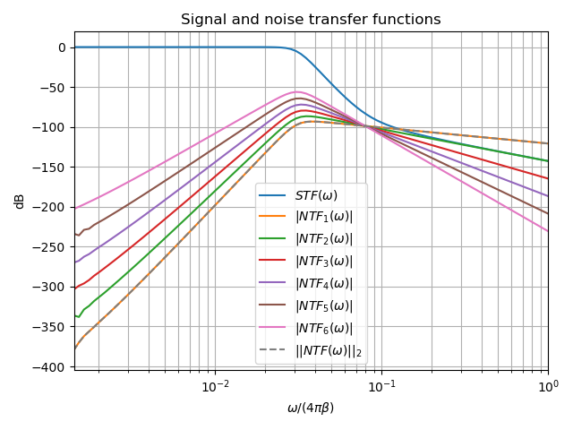
Visualize Estimator’s Transfer Function
132 # Logspace frequencies
133 frequencies = np.logspace(-3, 0, 100)
134 omega = 4 * np.pi * beta * frequencies
135
136 # Compute NTF
137 ntf = digital_estimator_ref.noise_transfer_function(omega)
138 ntf_dB = 20 * np.log10(np.abs(ntf))
139
140 # Compute STF
141 stf = digital_estimator_ref.signal_transfer_function(omega)
142 stf_dB = 20 * np.log10(np.abs(stf.flatten()))
143
144 # Signal attenuation at the input signal frequency
145 stf_at_omega = digital_estimator_ref.signal_transfer_function(
146     np.array([omega_3dB]))[0]
147
148 # Plot
149 plt.figure()
150 plt.semilogx(frequencies, stf_dB, label='$STF(\omega)$')
151 for n in range(N):
152     plt.semilogx(frequencies, ntf_dB[0, n, :], label=f"$|NTF_{n+1}(\omega)|$")
153 plt.semilogx(frequencies, 20 * np.log10(np.linalg.norm(
154     ntf[:, 0, :], axis=0)), '--', label="$ || NTF(\omega) ||_2 $")
155
156 # Add labels and legends to figure
157 plt.legend()
158 plt.grid(which='both')
159 plt.title("Signal and noise transfer functions")
160 plt.xlabel("$\omega / (4 \pi \\beta ) $")
161 plt.ylabel("dB")
162 plt.xlim((frequencies[5], frequencies[-1]))
163 plt.gcf().tight_layout()
Out:
/drives1/PhD/cbadc/docs/code_examples/b_general/plot_c_downsample.py:138: RuntimeWarning: divide by zero encountered in log10
  ntf_dB = 20 * np.log10(np.abs(ntf))
/drives1/PhD/cbadc/docs/code_examples/b_general/plot_c_downsample.py:153: RuntimeWarning: divide by zero encountered in log10
  plt.semilogx(frequencies, 20 * np.log10(np.linalg.norm(
FIR Filter With Downsampling
Next we repeat the initialization steps above but for a downsampled estimator
171 digital_estimator_dow = cbc.digital_estimator.FIRFilter(
172     analog_system,
173     digital_control,
174     eta2,
175     L1,
176     L2,
177     downsample=OSR)
178 digital_estimator_dow(control_signal_sequences2)
179
180 print(digital_estimator_dow, "\n")
Out:
FIR estimator is parameterized as
eta2 = 87574.26, 49 [dB],
Ts = 8e-05,
K1 = 4096,
K2 = 4096,
and
number_of_iterations = 9223372036854775808.
Resulting in the filter coefficients
h =
[[[ 3.55990445e-95  1.42412246e-95 -8.07811499e-96 -6.45762292e-97
    1.32955934e-96 -9.72617900e-98]
  [ 2.76240492e-95  1.82636990e-95 -7.62786724e-96 -1.33980733e-96
    1.38622941e-96 -1.24737454e-98]
  [ 1.76589627e-95  2.19922553e-95 -6.82068247e-96 -2.05614928e-96
    1.39325750e-96  8.21379656e-98]
  ...
  [ 1.76589627e-95 -2.16391013e-95 -7.69373510e-96  1.62200519e-96
    1.54381374e-96  4.50497165e-98]
  [ 2.76240492e-95 -1.77112250e-95 -8.34780716e-96  8.61459580e-97
    1.47844576e-96  1.38257124e-97]
  [ 3.55990446e-95 -1.35292339e-95 -8.63396392e-96  1.44959196e-97
    1.36586535e-96  2.17212387e-97]]].
Estimating (Filtering)
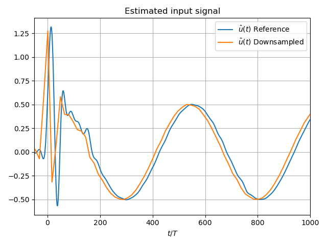
Aliasing
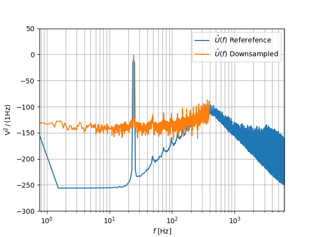
We compare the difference between the downsampled estimate and the default. Clearly, we are suffering from aliasing as is also explained by considering the PSD plot.
204 # compensate the built in L1 delay of FIR filter.
205 t = np.arange(-L1 + 1, size - L1 + 1)
206 t_down = np.arange(-(L1) // OSR, (size - L1) // OSR) * OSR + 1
207 plt.plot(t, u_hat_ref, label="$\hat{u}(t)$ Reference")
208 plt.plot(t_down, u_hat_dow, label="$\hat{u}(t)$ Downsampled")
209 plt.xlabel('$t / T$')
210 plt.legend()
211 plt.title("Estimated input signal")
212 plt.grid(which='both')
213 plt.xlim((-50, 1000))
214 plt.tight_layout()
215
216 plt.figure()
217 u_hat_ref_clipped = u_hat_ref[(L1 + L2):]
218 u_hat_dow_clipped = u_hat_dow[(L1 + L2) // OSR:]
219 f_ref, psd_ref = cbc.utilities.compute_power_spectral_density(
220     u_hat_ref_clipped, fs=1.0/T)
221 f_dow, psd_dow = cbc.utilities.compute_power_spectral_density(
222     u_hat_dow_clipped, fs=1.0/(T * OSR))
223 plt.semilogx(f_ref, 10 * np.log10(psd_ref), label="$\hat{U}(f)$ Referefence")
224 plt.semilogx(f_dow, 10 * np.log10(psd_dow), label="$\hat{U}(f)$ Downsampled")
225 plt.legend()
226 plt.ylim((-300, 50))
227 plt.xlim((f_ref[1], f_ref[-1]))
228 plt.xlabel('$f$ [Hz]')
229 plt.ylabel('$ \mathrm{V}^2 \, / \, (1 \mathrm{Hz})$')
230 plt.grid(which='both')
231 plt.show()
Out:
/home/hammal/anaconda3/envs/py38/lib/python3.8/site-packages/scipy/signal/spectral.py:1964: UserWarning: nperseg = 16384 is greater than input length  = 7680, using nperseg = 7680
  warnings.warn('nperseg = {0:d} is greater than input length '
Prepending a Virtual Bandlimiting Filter
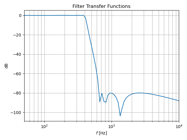
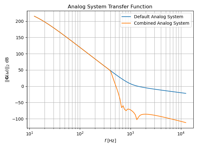
To battle the aliasing we extend the current estimator by placing a bandlimiting filter in front of the system. Note that this filter is a conceptual addition and not actually part of the physical analog system. Regardless, this effectively suppresses aliasing since we now reconstruct a signal shaped by both the STF of the system in addition to a bandlimiting filter.
245 wp = omega_3dB / 2.0
246 ws = omega_3dB
247 gpass = 0.1
248 gstop = 80
249
250 filter = cbc.analog_system.IIRDesign(wp, ws, gpass, gstop, ftype="ellip")
251
252 # Compute transfer functions for each frequency in frequencies
253 transfer_function_filter = filter.transfer_function_matrix(omega)
254
255 plt.semilogx(
256     omega/(2 * np.pi),
257     20 * np.log10(np.linalg.norm(
258         transfer_function_filter[:, 0, :],
259         axis=0)),
260     label="Cauer")
261 # Add labels and legends to figure
262 # plt.legend()
263 plt.grid(which='both')
264 plt.title("Filter Transfer Functions")
265 plt.xlabel("$f$ [Hz]")
266 plt.ylabel("dB")
267 plt.xlim((5e1, 1e4))
268 plt.gcf().tight_layout()
Out:
[6 3 5 2 4 1 0]
[3 0 4 1 5 2]
The analog system is parameterized as:
A =
[[ -158.38991952  2539.20594553]
 [-2539.20594553  -158.38991952]],
B =
[[1.30646843]
 [0.        ]],
CT =
[[  -316.77983904 -26439.53111383]],
Gamma =
None,
Gamma_tildeT =
None, and D=[[1.30646843]]
The analog system is parameterized as:
A =
[[ -507.42484717  2151.20032347]
 [-2151.20032347  -507.42484717]],
B =
[[1.30646843]
 [0.        ]],
CT =
[[-1014.84969433 -9539.6006361 ]],
Gamma =
None,
Gamma_tildeT =
None, and D=[[1.30646843]]
The analog system is parameterized as:
A =
[[ -872.67796009  1287.51180494]
 [-1287.51180494  -872.67796009]],
B =
[[1.30646843]
 [0.        ]],
CT =
[[ -1745.35592017 -12669.31428504]],
Gamma =
None,
Gamma_tildeT =
None, and D=[[1.30646843]]
The analog system is parameterized as:
A =
[[-1049.83492627]],
B =
[[1.1430085]],
CT =
[[1.]],
Gamma =
None,
Gamma_tildeT =
None, and D=[[0.]]
New Analog System
275 new_analog_system = cbc.analog_system.chain([filter, analog_system])
276 print(new_analog_system)
277
278 transfer_function_analog_system = analog_system.transfer_function_matrix(omega)
279
280 transfer_function_new_analog_system = new_analog_system.transfer_function_matrix(
281     omega)
282
283 plt.semilogx(
284     omega/(2 * np.pi),
285     20 * np.log10(np.linalg.norm(
286         transfer_function_analog_system[:, 0, :],
287         axis=0)),
288     label="Default Analog System")
289 plt.semilogx(
290     omega/(2 * np.pi),
291     20 * np.log10(np.linalg.norm(
292         transfer_function_new_analog_system[:, 0, :],
293         axis=0)),
294     label="Combined Analog System")
295
296 # Add labels and legends to figure
297 plt.legend()
298 plt.grid(which='both')
299 plt.title("Analog System Transfer Function")
300 plt.xlabel("$f$ [Hz]")
301 plt.ylabel("$||\mathbf{G}(\omega)||_2$ dB")
302 # plt.xlim((frequencies[0], frequencies[-1]))
303 plt.gcf().tight_layout()
Out:
The analog system is parameterized as:
A =
[[  -158.38991952   2539.20594553      0.              0.
       0.              0.              0.              0.
       0.              0.              0.              0.
       0.        ]
 [ -2539.20594553   -158.38991952      0.              0.
       0.              0.              0.              0.
       0.              0.              0.              0.
       0.        ]
 [  -413.86285921 -34542.41272467   -507.42484717   2151.20032347
       0.              0.              0.              0.
       0.              0.              0.              0.
       0.        ]
 [     0.              0.          -2151.20032347   -507.42484717
       0.              0.              0.              0.
       0.              0.              0.              0.
       0.        ]
 [  -540.69876022 -45128.57174752  -1325.86908763 -12463.18707325
    -872.67796009   1287.51180494      0.              0.
       0.              0.              0.              0.
       0.        ]
 [     0.              0.              0.              0.
   -1287.51180494   -872.67796009      0.              0.
       0.              0.              0.              0.
       0.        ]
 [  -618.0232788  -51582.34109438  -1515.47963687 -14245.52876018
   -1994.95665205 -14481.13391532  -1049.83492627      0.
       0.              0.              0.              0.
       0.        ]
 [     0.              0.              0.              0.
       0.              0.           6250.            -62.5
       0.              0.              0.              0.
       0.        ]
 [     0.              0.              0.              0.
       0.              0.              0.           6250.
     -62.5             0.              0.              0.
       0.        ]
 [     0.              0.              0.              0.
       0.              0.              0.              0.
    6250.            -62.5             0.              0.
       0.        ]
 [     0.              0.              0.              0.
       0.              0.              0.              0.
       0.           6250.            -62.5             0.
       0.        ]
 [     0.              0.              0.              0.
       0.              0.              0.              0.
       0.              0.           6250.            -62.5
       0.        ]
 [     0.              0.              0.              0.
       0.              0.              0.              0.
       0.              0.              0.           6250.
     -62.5       ]],
B =
[[1.30646843]
 [0.        ]
 [1.70685976]
 [0.        ]
 [2.22995839]
 [0.        ]
 [2.5488614 ]
 [0.        ]
 [0.        ]
 [0.        ]
 [0.        ]
 [0.        ]
 [0.        ]],
CT =
[[0. 0. 0. 0. 0. 0. 0. 1. 0. 0. 0. 0. 0.]
 [0. 0. 0. 0. 0. 0. 0. 0. 1. 0. 0. 0. 0.]
 [0. 0. 0. 0. 0. 0. 0. 0. 0. 1. 0. 0. 0.]
 [0. 0. 0. 0. 0. 0. 0. 0. 0. 0. 1. 0. 0.]
 [0. 0. 0. 0. 0. 0. 0. 0. 0. 0. 0. 1. 0.]
 [0. 0. 0. 0. 0. 0. 0. 0. 0. 0. 0. 0. 1.]],
Gamma =
[[    0.     0.     0.     0.     0.     0.]
 [    0.     0.     0.     0.     0.     0.]
 [    0.     0.     0.     0.     0.     0.]
 [    0.     0.     0.     0.     0.     0.]
 [    0.     0.     0.     0.     0.     0.]
 [    0.     0.     0.     0.     0.     0.]
 [    0.     0.     0.     0.     0.     0.]
 [-6250.    -0.    -0.    -0.    -0.    -0.]
 [   -0. -6250.    -0.    -0.    -0.    -0.]
 [   -0.    -0. -6250.    -0.    -0.    -0.]
 [   -0.    -0.    -0. -6250.    -0.    -0.]
 [   -0.    -0.    -0.    -0. -6250.    -0.]
 [   -0.    -0.    -0.    -0.    -0. -6250.]],
Gamma_tildeT =
[[0. 0. 0. 0. 0. 0. 0. 1. 0. 0. 0. 0. 0.]
 [0. 0. 0. 0. 0. 0. 0. 0. 1. 0. 0. 0. 0.]
 [0. 0. 0. 0. 0. 0. 0. 0. 0. 1. 0. 0. 0.]
 [0. 0. 0. 0. 0. 0. 0. 0. 0. 0. 1. 0. 0.]
 [0. 0. 0. 0. 0. 0. 0. 0. 0. 0. 0. 1. 0.]
 [0. 0. 0. 0. 0. 0. 0. 0. 0. 0. 0. 0. 1.]], and D=[[0.]
 [0.]
 [0.]
 [0.]
 [0.]
 [0.]]
New Digital Estimator
Combining the virtual pre filter together with the default analog system results in the following system.
312 digital_estimator_dow_and_pre_filt = cbc.digital_estimator.FIRFilter(
313     new_analog_system,
314     digital_control,
315     eta2,
316     L1,
317     L2,
318     downsample=OSR)
319 digital_estimator_dow_and_pre_filt(control_signal_sequences3)
320 print(digital_estimator_dow_and_pre_filt)
Out:
FIR estimator is parameterized as
eta2 = 87574.26, 49 [dB],
Ts = 8e-05,
K1 = 4096,
K2 = 4096,
and
number_of_iterations = 9223372036854775808.
Resulting in the filter coefficients
h =
[[[ 3.22671732e-26 -8.89499869e-27 -5.18313820e-27  1.64702740e-27
    8.08357583e-28 -2.46832942e-28]
  [ 3.62156532e-26 -6.14381653e-27 -5.93153659e-27  1.20605140e-27
    9.43071238e-28 -1.86905231e-28]
  [ 3.87168333e-26 -3.06068193e-27 -6.44545999e-27  7.02415336e-28
    1.04090230e-27 -1.17479413e-28]
  ...
  [-7.47293263e-25  2.48522571e-26  1.28642368e-25  4.66541431e-27
   -2.09696790e-26 -1.74944274e-27]
  [-7.47502086e-25 -3.86626172e-26  1.24250568e-25  1.51096568e-26
   -1.95583874e-26 -3.16125633e-27]
  [-7.16560992e-25 -9.90015793e-26  1.14790067e-25  2.46670037e-26
   -1.73669678e-26 -4.40656818e-27]]].
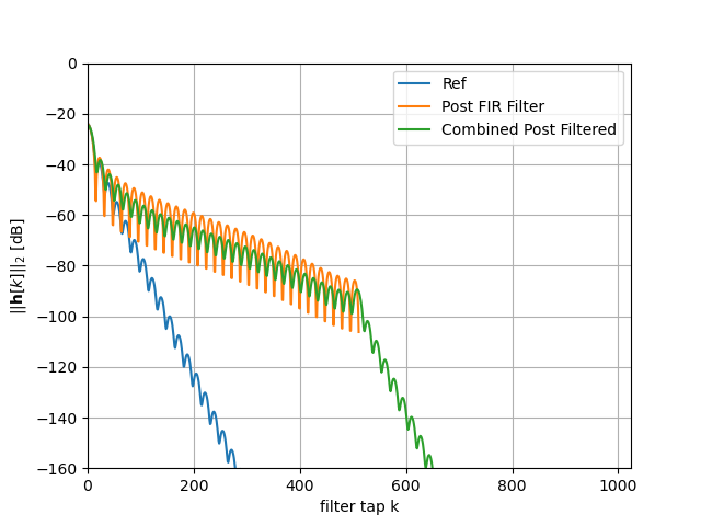
Post filtering the FIR filter coefficients
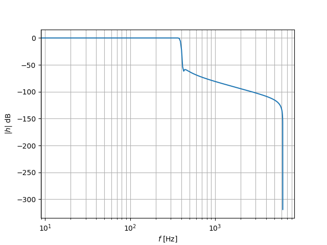
Yet another approach is to, instead of pre-filtering, post filter the resulting FIR filter coefficients with another lowpass FIR filter.
330 numtaps = 1 << 10
331 f_cutoff = 1.0 / OSR
332 fir_filter = scipy.signal.firwin(numtaps, f_cutoff)
333
334 digital_estimator_dow_and_post_filt = cbc.digital_estimator.FIRFilter(
335     analog_system,
336     digital_control,
337     eta2,
338     L1,
339     L2,
340     downsample=OSR)
341 digital_estimator_dow_and_post_filt(control_signal_sequences4)
342
343 # Apply the FIR post filter
344 digital_estimator_dow_and_post_filt.convolve(fir_filter)
345
346 print(digital_estimator_dow_and_post_filt, "\n")
347
348 FIR_frequency_response = np.fft.rfft(fir_filter)
349 f_FIR = np.fft.rfftfreq(numtaps, d=T)
350 plt.figure()
351 plt.semilogx(f_FIR, 20 * np.log10(np.abs(FIR_frequency_response)))
352 plt.xlabel('$f$ [Hz]')
353 plt.ylabel('$|h|$ dB')
354 plt.grid(which='both')
355
356 impulse_response_dB_dow = 20 * \
357     np.log10(np.linalg.norm(
358         np.array(digital_estimator_dow.h[0, :, :]), axis=1))
359
360 impulse_response_dB_dow_and_post_filt = 20 * \
361     np.log10(np.linalg.norm(
362         np.array(digital_estimator_dow_and_post_filt.h[0, :, :]), axis=1))
363
364 impulse_response_dB_FIR_filter = 20 * np.log10(np.abs(fir_filter[numtaps//2:]))
365
366 plt.figure()
367 plt.plot(np.arange(0, L1),
368          impulse_response_dB_dow[L1:],
369          label="Ref")
370 plt.plot(np.arange(0, numtaps//2),
371          impulse_response_dB_FIR_filter,
372          label="Post FIR Filter")
373 plt.plot(np.arange(0, L1),
374          impulse_response_dB_dow_and_post_filt[L1:],
375          label="Combined Post Filtered")
376
377 plt.legend()
378 plt.xlabel("filter tap k")
379 plt.ylabel("$|| \mathbf{h} [k]||_2$ [dB]")
380 plt.xlim((0, 1024))
381 plt.ylim((-160, 0))
382 plt.grid(which='both')
Out:
FIR estimator is parameterized as
eta2 = 87574.26, 49 [dB],
Ts = 8e-05,
K1 = 4096,
K2 = 4096,
and
number_of_iterations = 9223372036854775808.
Resulting in the filter coefficients
h =
[[[ 4.57908971e-87 -4.65114691e-87  1.82792564e-88  6.70779970e-88
   -1.47628062e-88 -6.91352512e-89]
  [ 6.94779186e-87 -4.67950396e-87 -1.70771451e-88  7.41295180e-88
   -1.07130519e-88 -8.41311065e-89]
  [ 9.29685994e-87 -4.52237142e-87 -5.56320514e-88  7.89684437e-88
   -5.78631185e-89 -9.73845893e-89]
  ...
  [ 1.15294566e-86  4.39630135e-87 -7.90611925e-88 -8.64551730e-88
   -6.70300573e-89  1.07217155e-88]
  [ 9.29685995e-87  4.70832786e-87 -3.71706891e-88 -8.17937370e-88
   -1.21559326e-88  9.13414714e-89]
  [ 6.94779186e-87  4.81847681e-87  1.92059492e-89 -7.46238158e-88
   -1.66273628e-88  7.37212989e-89]]].
Plotting the Estimator’s Signal and Noise Transfer Function
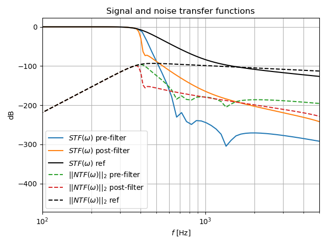
Next we visualize the resulting STF and NTF of the new digital estimator filters.
391 # Compute NTF
392 ntf_pre = digital_estimator_dow_and_pre_filt.noise_transfer_function(omega)
393 ntf_post = digital_estimator_dow_and_post_filt.noise_transfer_function(
394     2 * np.pi * f_FIR) * FIR_frequency_response
395 ntf_dow = digital_estimator_dow.noise_transfer_function(omega)
396
397 # Compute STF
398 stf_pre = digital_estimator_dow_and_pre_filt.signal_transfer_function(omega)
399 stf_dB_pre = 20 * np.log10(np.abs(stf_pre.flatten()))
400 stf_post = digital_estimator_dow_and_post_filt.signal_transfer_function(
401     2 * np.pi * f_FIR) * FIR_frequency_response
402 stf_dB_post = 20 * np.log10(np.abs(stf_post.flatten()))
403 stf_dow = digital_estimator_dow.signal_transfer_function(omega)
404 stf_dow_dB = 20 * np.log10(np.abs(stf_dow.flatten()))
405
406 # Plot
407 plt.figure()
408 plt.semilogx(omega/(2 * np.pi), stf_dB_pre, label='$STF(\omega)$ pre-filter')
409 plt.semilogx(f_FIR, stf_dB_post, label='$STF(\omega)$ post-filter')
410 plt.semilogx(omega/(2 * np.pi), stf_dow_dB,
411              label='$STF(\omega)$ ref',  color='black')
412 plt.semilogx(omega/(2 * np.pi), 20 * np.log10(np.linalg.norm(
413     ntf_pre[:, 0, :], axis=0)), '--', label="$ || NTF(\omega) ||_2 $ pre-filter")
414 plt.semilogx(f_FIR, 20 * np.log10(np.linalg.norm(
415     ntf_post[:, 0, :], axis=0)), '--', label="$ || NTF(\omega) ||_2 $ post-filter")
416 plt.semilogx(omega/(2 * np.pi), 20 * np.log10(np.linalg.norm(
417     ntf_dow[:, 0, :], axis=0)), '--', label="$ || NTF(\omega) ||_2 $ ref", color='black')
418
419 # Add labels and legends to figure
420 plt.legend()
421 plt.grid(which='both')
422 plt.title("Signal and noise transfer functions")
423 plt.xlabel("$f$ [Hz]")
424 plt.ylabel("dB")
425 plt.xlim((1e2, 5e3))
426 plt.gcf().tight_layout()
Out:
/drives1/PhD/cbadc/docs/code_examples/b_general/plot_c_downsample.py:412: RuntimeWarning: divide by zero encountered in log10
  plt.semilogx(omega/(2 * np.pi), 20 * np.log10(np.linalg.norm(
/drives1/PhD/cbadc/docs/code_examples/b_general/plot_c_downsample.py:416: RuntimeWarning: divide by zero encountered in log10
  plt.semilogx(omega/(2 * np.pi), 20 * np.log10(np.linalg.norm(
Filtering Estimate
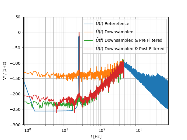
Finally, we plot the resulting input estimate PSD for each estimator. Clearly, both the pre and post filter effectively suppresses the aliasing effect.
437 u_hat_dow_and_pre_filt = np.zeros(size // OSR)
438 u_hat_dow_and_post_filt = np.zeros(size // OSR)
439 for index in cbc.utilities.show_status(range(size // OSR)):
440     u_hat_dow_and_pre_filt[index] = next(digital_estimator_dow_and_pre_filt)
441     u_hat_dow_and_post_filt[index] = next(digital_estimator_dow_and_post_filt)
442
443 plt.figure()
444 u_hat_dow_and_pre_filt_clipped = u_hat_dow_and_pre_filt[(L1 + L2) // OSR:]
445 u_hat_dow_and_post_filt_clipped = u_hat_dow_and_post_filt[(L1 + L2) // OSR:]
446 _, psd_dow_and_pre_filt = cbc.utilities.compute_power_spectral_density(
447     u_hat_dow_and_pre_filt_clipped, fs=1.0/(T * OSR))
448 _, psd_dow_and_post_filt = cbc.utilities.compute_power_spectral_density(
449     u_hat_dow_and_post_filt_clipped, fs=1.0/(T * OSR))
450 plt.semilogx(f_ref, 10 * np.log10(psd_ref), label="$\hat{U}(f)$ Referefence")
451 plt.semilogx(f_dow, 10 * np.log10(psd_dow), label="$\hat{U}(f)$ Downsampled")
452 plt.semilogx(f_dow, 10 * np.log10(psd_dow_and_pre_filt),
453              label="$\hat{U}(f)$ Downsampled & Pre Filtered")
454 plt.semilogx(f_dow, 10 * np.log10(psd_dow_and_post_filt),
455              label="$\hat{U}(f)$ Downsampled & Post Filtered")
456 plt.legend()
457 plt.ylim((-300, 50))
458 plt.xlim((f_ref[1], f_ref[-1]))
459 plt.xlabel('$f$ [Hz]')
460 plt.ylabel('$ \mathrm{V}^2 \, / \, (1 \mathrm{Hz})$')
461 plt.grid(which='both')
462 plt.show()
Out:
  0%|          | 0/8192 [00:00<?, ?it/s]
  1%|1         | 112/8192 [00:00<00:07, 1113.18it/s]
  3%|2         | 224/8192 [00:00<00:08, 971.98it/s]
  4%|3         | 323/8192 [00:00<00:11, 683.12it/s]
  5%|5         | 441/8192 [00:00<00:09, 828.53it/s]
  7%|7         | 581/8192 [00:00<00:07, 996.57it/s]
  9%|8         | 732/8192 [00:00<00:06, 1148.64it/s]
 11%|#         | 867/8192 [00:00<00:06, 1208.21it/s]
 12%|#2        | 1003/8192 [00:00<00:05, 1251.68it/s]
 14%|#4        | 1156/8192 [00:01<00:05, 1333.60it/s]
 16%|#5        | 1309/8192 [00:01<00:04, 1391.13it/s]
 18%|#7        | 1451/8192 [00:01<00:05, 1224.73it/s]
 19%|#9        | 1579/8192 [00:01<00:06, 1045.88it/s]
 21%|##        | 1692/8192 [00:01<00:07, 919.74it/s]
 22%|##2       | 1822/8192 [00:01<00:06, 1006.86it/s]
 24%|##4       | 1968/8192 [00:01<00:05, 1118.29it/s]
 26%|##5       | 2119/8192 [00:01<00:04, 1219.79it/s]
 28%|##7       | 2264/8192 [00:02<00:04, 1280.42it/s]
 29%|##9       | 2398/8192 [00:02<00:04, 1286.40it/s]
 31%|###1      | 2550/8192 [00:02<00:04, 1351.67it/s]
 33%|###2      | 2701/8192 [00:02<00:03, 1396.58it/s]
 35%|###4      | 2855/8192 [00:02<00:03, 1436.18it/s]
 37%|###6      | 3008/8192 [00:02<00:03, 1463.59it/s]
 39%|###8      | 3156/8192 [00:02<00:04, 1148.15it/s]
 40%|####      | 3283/8192 [00:02<00:04, 1112.00it/s]
 42%|####1     | 3435/8192 [00:02<00:03, 1214.27it/s]
 44%|####3     | 3566/8192 [00:03<00:03, 1237.90it/s]
 45%|####5     | 3708/8192 [00:03<00:03, 1286.44it/s]
 47%|####6     | 3849/8192 [00:03<00:03, 1319.64it/s]
 49%|####8     | 3994/8192 [00:03<00:03, 1352.35it/s]
 51%|#####     | 4140/8192 [00:03<00:02, 1381.55it/s]
 52%|#####2    | 4287/8192 [00:03<00:02, 1407.29it/s]
 54%|#####4    | 4430/8192 [00:03<00:02, 1343.64it/s]
 56%|#####5    | 4583/8192 [00:03<00:02, 1395.13it/s]
 58%|#####7    | 4734/8192 [00:03<00:02, 1426.86it/s]
 60%|#####9    | 4880/8192 [00:03<00:02, 1436.48it/s]
 61%|######1   | 5025/8192 [00:04<00:02, 1357.78it/s]
 63%|######3   | 5177/8192 [00:04<00:02, 1403.46it/s]
 65%|######5   | 5330/8192 [00:04<00:01, 1437.53it/s]
 67%|######6   | 5483/8192 [00:04<00:01, 1463.92it/s]
 69%|######8   | 5636/8192 [00:04<00:01, 1481.27it/s]
 71%|#######   | 5785/8192 [00:04<00:01, 1479.85it/s]
 72%|#######2  | 5934/8192 [00:04<00:01, 1374.40it/s]
 74%|#######4  | 6087/8192 [00:04<00:01, 1417.25it/s]
 76%|#######6  | 6231/8192 [00:04<00:01, 1224.62it/s]
 78%|#######7  | 6359/8192 [00:05<00:01, 1182.20it/s]
 79%|#######9  | 6481/8192 [00:05<00:01, 1173.80it/s]
 81%|########  | 6613/8192 [00:05<00:01, 1212.94it/s]
 83%|########2 | 6764/8192 [00:05<00:01, 1294.61it/s]
 84%|########4 | 6897/8192 [00:05<00:00, 1303.56it/s]
 86%|########5 | 7029/8192 [00:05<00:00, 1212.83it/s]
 88%|########7 | 7181/8192 [00:05<00:00, 1296.77it/s]
 90%|########9 | 7334/8192 [00:05<00:00, 1362.52it/s]
 91%|#########1| 7487/8192 [00:05<00:00, 1410.08it/s]
 93%|#########3| 7639/8192 [00:06<00:00, 1441.75it/s]
 95%|#########5| 7791/8192 [00:06<00:00, 1462.65it/s]
 97%|#########6| 7939/8192 [00:06<00:00, 1312.53it/s]
 99%|#########8| 8092/8192 [00:06<00:00, 1369.76it/s]
100%|##########| 8192/8192 [00:06<00:00, 1275.08it/s]
/home/hammal/anaconda3/envs/py38/lib/python3.8/site-packages/scipy/signal/spectral.py:1964: UserWarning: nperseg = 16384 is greater than input length  = 7680, using nperseg = 7680
  warnings.warn('nperseg = {0:d} is greater than input length '
In Time Domain
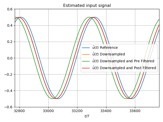
The corresponding estimate samples are plotted. As is evident from the plots the different filter realization all result in different filter lags. Naturally, the filter lag follows from the choice of K1, K2, and the pre or post filter design and is therefore a known parameter.
473 t = np.arange(size)
474 t_down = np.arange(size // OSR) * OSR
475 plt.plot(t, u_hat_ref, label="$\hat{u}(t)$ Reference")
476 plt.plot(t_down, u_hat_dow, label="$\hat{u}(t)$ Downsampled")
477 plt.plot(t_down, u_hat_dow_and_pre_filt,
478          label="$\hat{u}(t)$ Downsampled and Pre Filtered")
479 plt.plot(t_down, u_hat_dow_and_post_filt,
480          label="$\hat{u}(t)$ Downsampled and Post Filtered")
481 plt.xlabel('$t / T$')
482 plt.legend()
483 plt.title("Estimated input signal")
484 plt.grid(which='both')
485 offset = (L1 + L2) * 4
486 plt.xlim((offset, offset + 1000))
487 plt.ylim((-0.6, 0.6))
488 plt.tight_layout()
Compare Filter Coefficients
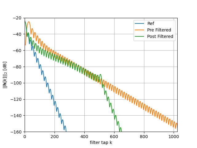
Futhermore, the filter coefficient’s magnitude decay varies for the different implementations. Keep in mind that the for this example the pre and post filter are parametrized such that the formed slightly outperforms the latter in terms of precision (see the PSD plot above).
499 impulse_response_dB_dow_and_pre_filt = 20 * \
500     np.log10(np.linalg.norm(
501         np.array(digital_estimator_dow_and_pre_filt.h[0, :, :]), axis=1))
502
503 plt.plot(np.arange(0, L1),
504          impulse_response_dB_dow[L1:],
505          label="Ref")
506
507 plt.plot(np.arange(0, L1),
508          impulse_response_dB_dow_and_pre_filt[L1:],
509          label="Pre Filtered")
510 plt.plot(np.arange(0, L1),
511          impulse_response_dB_dow_and_post_filt[L1:],
512          label="Post Filtered")
513 plt.legend()
514 plt.xlabel("filter tap k")
515 plt.ylabel("$|| \mathbf{h} [k]||_2$ [dB]")
516 plt.xlim((0, 1024))
517 plt.ylim((-160, -20))
518 plt.grid(which='both')
Total running time of the script: ( 1 minutes 23.417 seconds)