Loading a Hadamard Ramp Simulation

Builds on…

import cbadc
import cbadc.datasets.hadamard
import scipy.signal
import numpy as np
import matplotlib.pyplot as plt

Create a Simulation Wrapper

We load the PCB A prototype by instantiating the wrapper class as

simulation_wrapper = cbadc.datasets.hadamard.HadamardPCB('B')

Load a specific simulation

In this case we load cbadc.datasets.hadamard.HadamardPCB.simulation_ramp_1_B() simulation by invoking

control_signal, ideal_control_signal, simulator, size = simulation_wrapper.simulation_ramp_1_B()

size = 1 << 12

Configure a Digital Estimator

eta2 = 1e5
L1 = 1 << 10
L2 = 1 << 10
OSR = 1 << 5


digital_estimator = cbadc.digital_estimator.FIRFilter(
    simulator.analog_system,
    simulator.digital_control,
    eta2,
    L1,
    L2,
    downsample=OSR)

print(digital_estimator, "\n")

digital_estimator(control_signal)

Out:

FIR estimator is parameterized as
eta2 = 100000.00, 50 [dB],
Ts = 1e-06,
K1 = 1024,
K2 = 1024,
and
number_of_iterations = 9223372036854775808.
Resulting in the filter coefficients
h =
[[[-1.78705424e-11  3.59873868e-12  6.75066574e-13 ...  5.09395743e-12
    3.63212138e-12  5.64068310e-12]
  [-1.85063565e-11  3.47173121e-12  7.55741807e-13 ...  5.19952008e-12
    3.84152538e-12  5.78952380e-12]
  [-1.91180522e-11  3.33009324e-12  8.37677092e-13 ...  5.29530790e-12
    4.04909983e-12  5.92876483e-12]
  ...
  [-1.91180522e-11 -3.33009324e-12  8.37677092e-13 ...  3.84487966e-12
    5.92876483e-12  4.04909983e-12]
  [-1.85063565e-11 -3.47173121e-12  7.55741807e-13 ...  3.67578729e-12
    5.78952380e-12  3.84152538e-12]
  [-1.78705424e-11 -3.59873868e-12  6.75066574e-13 ...  3.50378048e-12
    5.64068310e-12  3.63212138e-12]]].

Post filtering with FIR

numtaps = 1 << 10
f_cutoff = 1.0 / OSR
fir_filter = scipy.signal.firwin(numtaps, f_cutoff)

digital_estimator.convolve((fir_filter))

Filtering Estimate

u_hat = np.zeros(size // OSR)
for index in cbadc.utilities.show_status(range(size // OSR)):
    u_hat[index] = next(digital_estimator)

Out:

  0%|          | 0/128 [00:00<?, ?it/s]
  1%|          | 1/128 [00:00<01:06,  1.91it/s]
 76%|#######5  | 97/128 [00:00<00:00, 207.19it/s]
100%|##########| 128/128 [00:00<00:00, 194.49it/s]

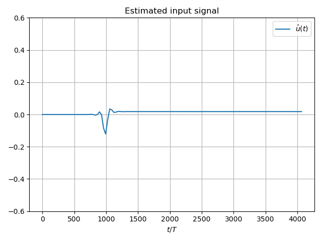
Visualize Estimate

t = np.arange(size // OSR) * OSR
plt.plot(t, u_hat, label="$\hat{u}(t)$")
plt.xlabel('$t / T$')
plt.legend()
plt.title("Estimated input signal")
plt.grid(which='both')
# offset = (L1 + L2) * 4
# plt.xlim((offset, offset + 1000))
plt.ylim((-0.6, 0.6))
plt.tight_layout()

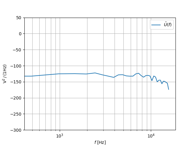
Visualize Estimate Spectrum

plt.figure()
u_hat_clipped = u_hat[(L1 + L2) // OSR:]
freq, psd = cbadc.utilities.compute_power_spectral_density(
    u_hat_clipped, fs=1.0/(simulator.digital_control.T * OSR))
plt.semilogx(freq, 10 * np.log10(psd), label="$\hat{U}(f)$")
plt.legend()
plt.ylim((-300, 50))
# plt.xlim((f_ref[1], f_ref[-1]))
plt.xlabel('$f$ [Hz]')
plt.ylabel('$ \mathrm{V}^2 \, / \, (1 \mathrm{Hz})$')
plt.grid(which='both')
plt.show()

Out:

/home/hammal/anaconda3/envs/py38/lib/python3.8/site-packages/scipy/signal/spectral.py:1964: UserWarning: nperseg = 16384 is greater than input length  = 64, using nperseg = 64
  warnings.warn('nperseg = {0:d} is greater than input length '